We review the basic properties of power series representation of functions.
Review of Power Series
Many applications give rise to differential equations with solutions that can’t be expressed in terms of elementary functions such as polynomials, rational functions, exponential and logarithmic functions, and trigonometric functions. The solutions of some of the most important of these equations can be expressed in terms of power series. We’ll study such equations in this chapter. In this section we review relevant properties of power series. We’ll omit proofs, which can be found in any standard calculus text.
A power series in must converge if , since the positive powers of are all zero in this case. This may be the only value of for which the power series converges. However, the next theorem shows that if the power series converges for some then the set of all values of for which it converges forms an interval.
In case item:7.1.2c we say that is the radius of convergence of the power series. For convenience, we include the other two cases in this definition by defining in case item:7.1.2a and in case item:7.1.2b. We define the open interval of convergence of to be If is finite, no general statement can be made concerning convergence at the endpoints of the open interval of convergence; the series may converge at one or both points, or diverge at both.
Recall from calculus that a series of constants is said to converge absolutely if the series of absolute values converges. It can be shown that a power series with a positive radius of convergence converges absolutely in its open interval of convergence; that is, the series of absolute values converges if . However, if , the series may fail to converge absolutely at an endpoint , even if it converges there.
The next theorem provides a useful method for determining the radius of convergence of a power series. It’s derived in calculus by applying the ratio test to the corresponding series of absolute values.
Taylor Series
If a function has derivatives of all orders at a point , then the Taylor series of about is defined by In the special case where , this series is also called the Maclaurin series of .
Taylor series for most of the common elementary functions converge to the functions on their open intervals of convergence. For example, you are probably familiar with the following Maclaurin series:
Differentiation of Power Series
A power series with a positive radius of convergence defines a function on its open interval of convergence. We say that the series represents on the open interval of convergence. A function represented by a power series may be a familiar elementary function as in (eq:7.1.2)–(eq:7.1.5); however, it often happens that isn’t a familiar function, so the series actually defines .
The next theorem shows that a function represented by a power series has derivatives of all orders on the open interval of convergence of the power series, and provides power series representations of the derivatives.
Uniqueness of Power Series
The next theorem shows that if is defined by a power series in with a positive radius of convergence, then the power series is the Taylor series of about .
This result can be obtained by setting in (eq:7.1.8), which yields This implies that Except for notation, this is the same as (eq:7.1.9).
The next theorem lists two important properties of power series that follow from Theorem thmtype:7.1.5.
To obtain item:7.1.6a we observe that the two series represent the same function on the open interval; hence, Theorem thmtype:7.1.5 implies that Part item:7.1.6b can be obtained from item:7.1.6a by taking for .
Taylor Polynomials
If has derivatives at a point , we say that is the -th Taylor polynomial of about . This definition and Theorem thmtype:7.1.5 imply that if where the power series has a positive radius of convergence, then the Taylor polynomials of about are given by In numerical applications, we use the Taylor polynomials to approximate on subintervals of the open interval of convergence of the power series. For example, (eq:7.1.2) implies that the Taylor polynomial of is The solid curve in the figure below is the graph of on the interval . The dotted curves in the figure are the graphs of the Taylor polynomials of about .
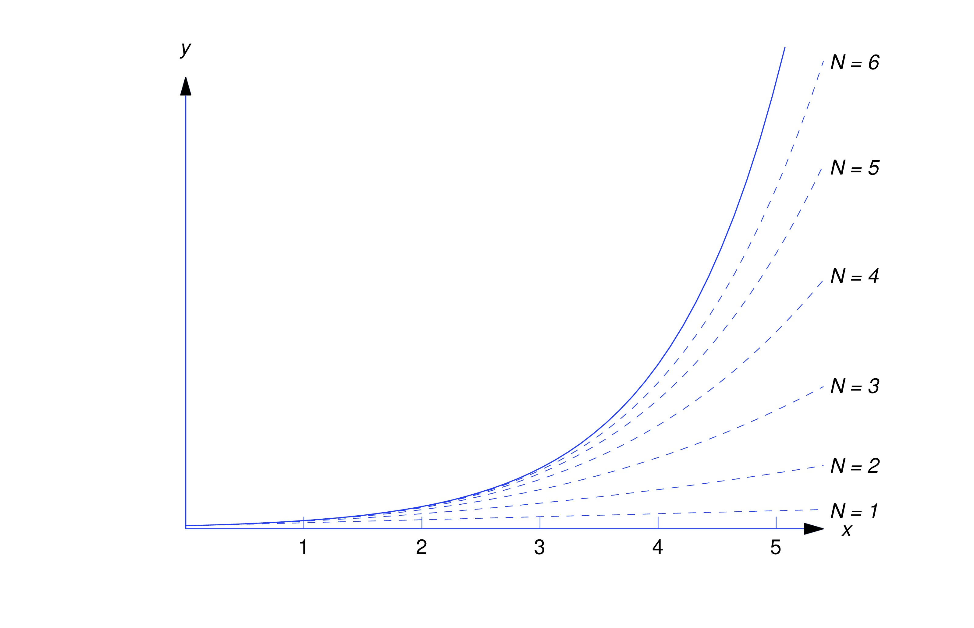
From this figure, we conclude that the accuracy of the approximation of by its Taylor polynomial improves as increases.
Shifting the Summation Index
In Definition thmtype:7.1.1 of a power series in , the -th term is a constant multiple of . This isn’t true in (eq:7.1.6), (eq:7.1.7), and (eq:7.1.8), where the general terms are constant multiples of , , and , respectively. However, these series can all be rewritten so that their -th terms are constant multiples of . For example, letting in the series in (eq:7.1.6) yields
where we start the new summation index from zero so that the first term in (eq:7.1.10) (obtained by setting ) is the same as the first term in (eq:7.1.6) (obtained by setting ). However, the sum of a series is independent of the symbol used to denote the summation index, just as the value of a definite integral is independent of the symbol used to denote the variable of integration. Therefore we can replace by in (eq:7.1.10) to obtain where the general term is a constant multiple of .It isn’t really necessary to introduce the intermediate summation index . We can obtain (eq:7.1.11) directly from (eq:7.1.6) by replacing by in the general term of (eq:7.1.6) and subtracting from the lower limit of (eq:7.1.6). More generally, we use the following procedure for shifting indices.
For any integer , the power series can be rewritten as that is, replacing by in the general term and subtracting from the lower limit of summation leaves the series unchanged.
item:7.1.3b Replacing by in the general term and subtracting from the lower limit of summation yields
Linear Combinations of Power Series
If a power series is multiplied by a constant, then the constant can be placed inside the summation; that is, Two power series with positive radii of convergence can be added term by term at points common to their open intervals of convergence; thus, if the first series converges for and the second converges for , then for , where is the smaller of and . More generally, linear combinations of power series can be formed term by term; for example,
- (a)
- Express as a power series in on .
- (b)
- Use the result of item:ex7.1.6a to find necessary and sufficient conditions on the coefficients for to be a solution of the homogeneous equation on .
item:ex7.1.6b From (eq:7.1.17) we see that satisfies (eq:7.1.13) on if
Conversely, Theorem thmtype:7.1.6 item:7.1.6b implies that if satisfies (eq:7.1.13) on , then (eq:7.1.18) holds.Text Source
Trench, William F., ”Elementary Differential Equations” (2013). Faculty Authored and Edited Books & CDs. 8. (CC-BY-NC-SA)