Need an abstract
Transformation of Homogeneous Equations into Separable Equations
Nonlinear Equations That Can be Transformed Into Separable Equations
We’ve seen that the nonlinear Bernoulli equation can be transformed into a separable equation by the substitution if is suitably chosen. Now let’s discover a sufficient condition for a nonlinear first order differential equation
to be transformable into a separable equation in the same way. Substituting into (eq:2.4.4) yields which is equivalent to If for some function , then (eq:2.4.5) becomes which is separable. After checking for constant solutions such that , we can separate variables to obtainHomogeneous Nonlinear Equations
In the text we’ll consider only the most widely studied class of equations for which the method of the preceding paragraph works. Other types of equations appear in Exercises exer:2.4.44–exer:2.4.51.
The differential equation (eq:2.4.4) is said to be homogeneous if and occur in in such a way that depends only on the ratio ; that is, (eq:2.4.4) can be written as
where is a function of a single variable. For example, and are of the form (eq:2.4.7), with respectively. The general method discussed above can be applied to (eq:2.4.7) with (and therefore . Thus, substituting in (eq:2.4.7) yields and separation of variables (after checking for constant solutions such that ) yieldsBefore turning to examples, we point out something that you may’ve have already noticed: the definition of homogeneous equation given here isn’t the same as the definition given in Section 2.1, where we said that a linear equation of the form is homogeneous. We make no apology for this inconsistency, since we didn’t create it! Historically, homogeneous has been used in these two inconsistent ways. The one having to do with linear equations is the most important. This is the only section of the book where the meaning defined here will apply.
Since is in general undefined if , we’ll consider solutions of nonhomogeneous equations only on open intervals that do not contain the point .
Substituting into (eq:2.4.8) yields Simplifying and separating variables yields Integrating yields . Therefore and .
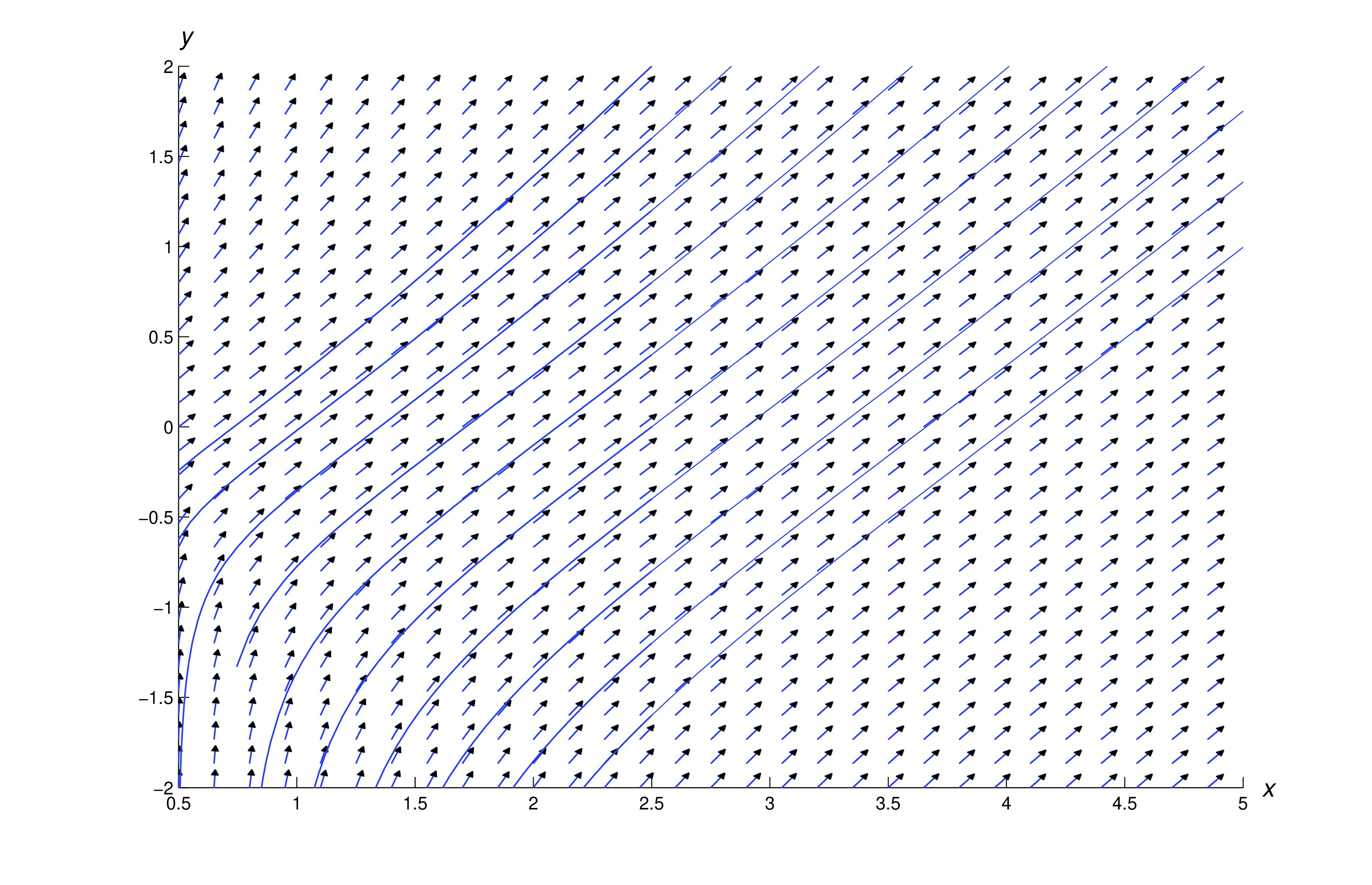
Figure figure:2.4.2 shows a direction field and integral curves for (eq:2.4.8).
Therefore
is a solution of (eq:2.4.10) for any choice of the constant . Setting in (eq:2.4.13) yields the solution . However, the solution can’t be obtained from (eq:2.4.13). Thus, the solutions of (eq:2.4.9) on intervals that don’t contain are and functions of the form (eq:2.4.13).The situation is more complicated if is the open interval. First, note that satisfies (eq:2.4.9) on . If and are arbitrary constants, the function
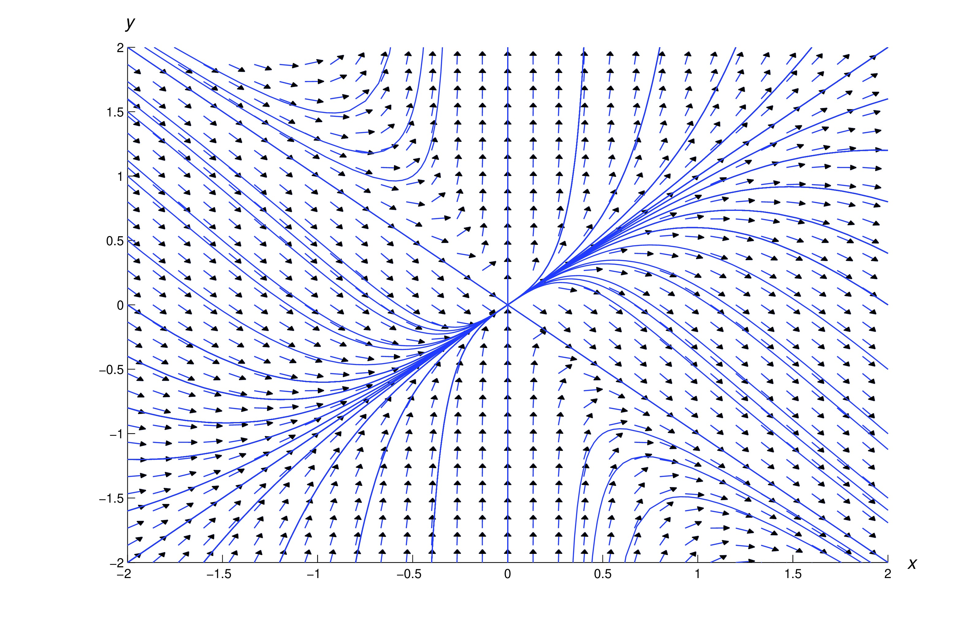
is a solution of (eq:2.4.9) on , where We leave it to you to verify this. To do so, note that if is any function of the form (eq:2.4.13) then and .Figure figure:2.4.3 shows a direction field and some integral curves for (eq:2.4.9).
example:2.4.3b We could obtain by imposing the initial condition in (eq:2.4.13), and then solving for . However, it’s easier to use (eq:2.4.12). Since , the initial condition implies that . Substituting this into (eq:2.4.12) yields . Hence, the solution of (eq:2.4.10) is The interval of validity of this solution is . However, the largest interval on which (eq:2.4.10) has a unique solution is . To see this, note from (eq:2.4.14) that any function of the form
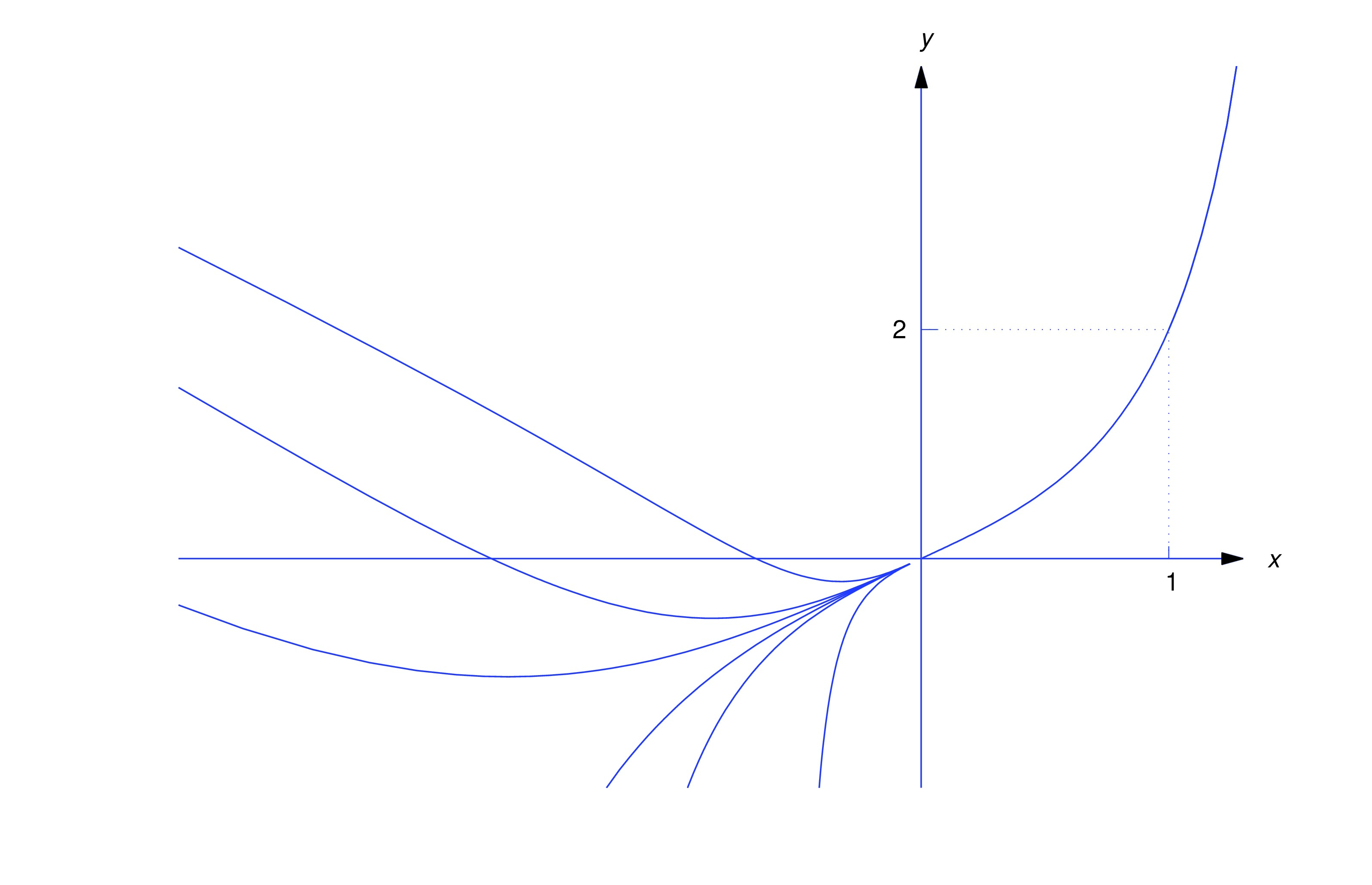
is a solution of (eq:2.4.10) on , where if or if . (Why doesn’t this contradict Theorem thmtype:2.3.1?)Figure figure:2.4.4 shows several solutions of the initial value problem (eq:2.4.10). Note that these solutions coincide on .
In the last two examples we were able to solve the given equations explicitly. However, this isn’t always possible, as you’ll see if you attempt the exercises in Trench, Section 2.4.