We define autonomous equations, explain how autonomous second order equations can be reduced to first order equations, and give several applications.
Autonomous Second Order Equations
A second order differential equation that can be written as
where is independent of , is said to be autonomous. An autonomous second order equation can be converted into a first order equation relating and . If we let , (eq:4.4.1) becomes Since (eq:4.4.2) can be rewritten as The integral curves of (eq:4.4.4) can be plotted in the plane, which is called the Poincaré phase plane of (eq:4.4.1). If is a solution of (eq:4.4.1) then is a parametric equation for an integral curve of (eq:4.4.4). We’ll call these integral curves trajectories of (eq:4.4.1), and we’ll call (eq:4.4.4) the phase plane equivalent of (eq:4.4.1).In this section we’ll consider autonomous equations that can be written as
Equations of this form often arise in applications of Newton’s second law of motion. For example, suppose is the displacement of a moving object with mass . It’s reasonable to think of two types of time-independent forces acting on the object. One type - such as gravity - depends only on position. We could write such a force as . The second type - such as atmospheric resistance or friction - may depend on position and velocity. (Forces that depend on velocity are called damping forces.) We write this force as , where is usually a positive function and we’ve put the factor outside to make it explicit that the force is in the direction opposing the motion. In this case Newton’s, second law of motion leads to (eq:4.4.5).The phase plane equivalent of (eq:4.4.5) is
Some statements that we’ll be making about the properties of (eq:4.4.5) and (eq:4.4.6) are intuitively reasonable, but difficult to prove. Therefore our presentation in this section will be informal: we’ll just say things without proof, all of which are true if we assume that is continuously differentiable for all and is continuously differentiable for all . We begin with the following statements:Statement 1. If and are arbitrary real numbers then (eq:4.4.5) has a unique solution on such that and .
Statement 2. If is a solution of (eq:4.4.5) and is any constant then is also a solution of (eq:4.4.5), and and have the same trajectory.
Statement 3. If two solutions and of (eq:4.4.5) have the same trajectory then for some constant .
Statement 4. Distinct trajectories of (eq:4.4.5) can’t intersect; that is, if two trajectories of (eq:4.4.5) intersect, they are identical.
Statement 5. If the trajectory of a solution of (eq:4.4.5) is a closed curve then traverses the trajectory in a finite time , and the solution is periodic with period ; that is, for all in .
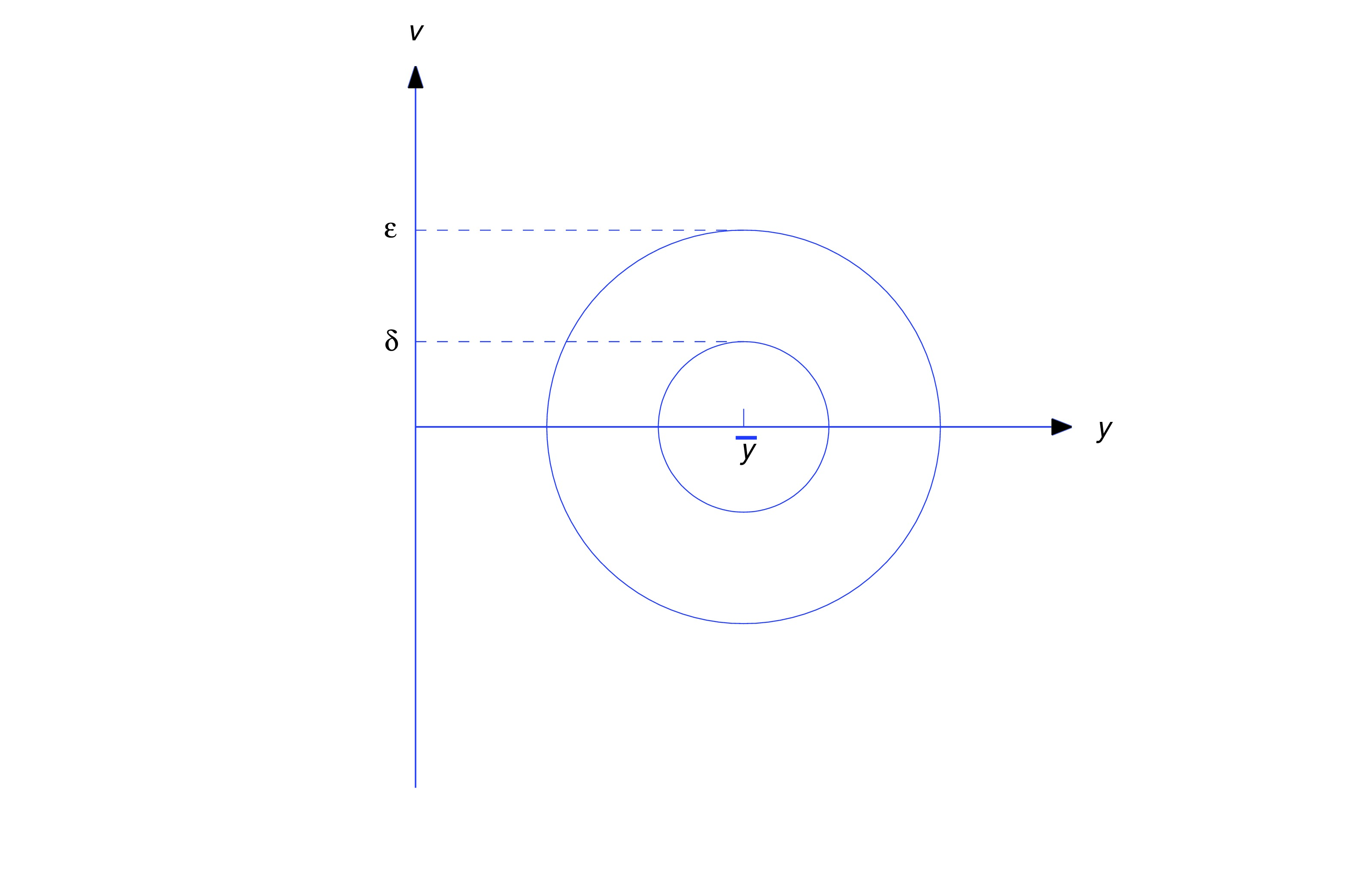
If is a constant such that then is a constant solution of (eq:4.4.5). We say that is an equilibrium of (eq:4.4.5) and is a critical point of the phase plane equivalent equation (eq:4.4.6). We say that the equilibrium and the critical point are stable if, for any given no matter how small, there’s a , sufficiently small, such that if then the solution of the initial value problem satisfies the inequality for all . The figure below illustrates the geometrical interpretation of this definition in the Poincaré phase plane: if is in the smaller shaded circle (with radius ), then must be in in the larger circle (with radius ) for all .
If an equilibrium and the associated critical point are not stable, we say they are unstable. To see if you really understand what stable means, try to give a direct definition of unstable We’ll illustrate both definitions in the following examples.
The Undamped Case
We’ll begin with the case where , so (eq:4.4.5) reduces to
We say that this equation - as well as any physical situation that it may model - is undamped. The phase plane equivalent of (eq:4.4.7) is the separable equation Integrating this yields where is a constant of integration and is an antiderivative of .If (eq:4.4.7) is the equation of motion of an object of mass , then is the kinetic energy and is the potential energy of the object; thus, (eq:4.4.8) says that the total energy of the object remains constant, or is conserved. In particular, if a trajectory passes through a given point then
Assume that if the length of the spring is changed by an amount (positive or negative), then the spring exerts an opposing force with magnitude , where k is a positive constant. In Trench 6.1 it will be shown that if the mass of the spring is negligible compared to and no other forces act on the object then Newton’s second law of motion implies that
which can be written in the form (eq:4.4.7) with . This equation can be solved easily by a method that we’ll study in Trench 5.1, but that method isn’t available here. Instead, we’ll consider the phase plane equivalent of (eq:4.4.9).From (eq:4.4.3), we can rewrite (eq:4.4.9) as the separable equation Integrating this yields which implies that
(). This defines an ellipse in the Poincaré phase plane.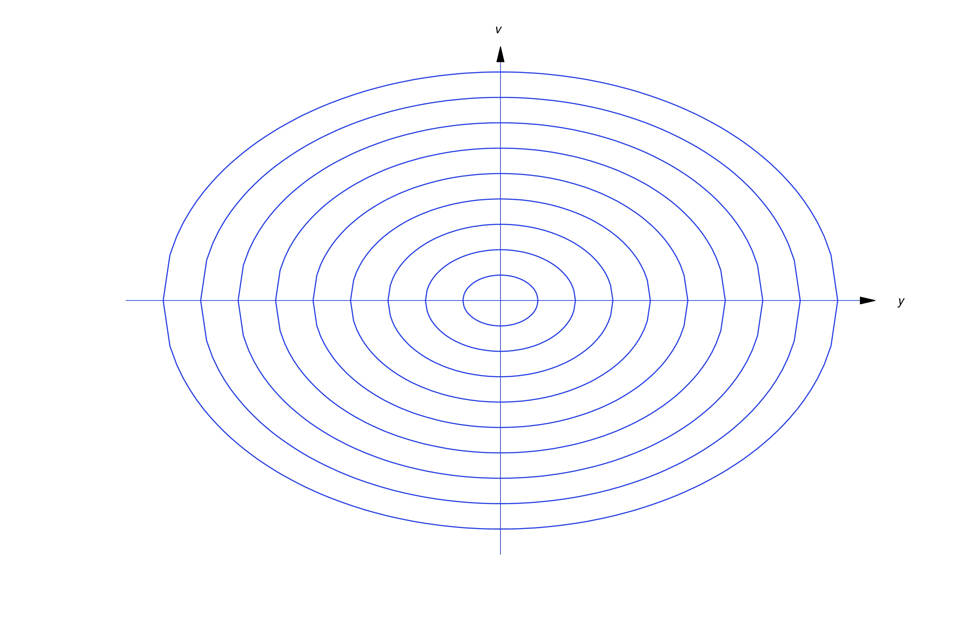
We can identify by setting in (eq:4.4.10); thus, , where and . To determine the maximum and minimum values of we set in (eq:4.4.10); thus,
Equation (eq:4.4.9) has exactly one equilibrium, , and it’s stable. You can see intuitively why this is so: if the object is displaced in either direction from equilibrium, the spring tries to bring it back.In this case we can find explicitly as a function of . (Don’t expect this to happen in more complicated problems!) If on an interval , (eq:4.4.10) implies that on . This is equivalent to
Since (see (eq:4.4.11)), (eq:4.4.12) implies that that there’s a constant such that or for all in . Although we obtained this function by assuming that , you can easily verify that satisfies (eq:4.4.9) for all values of . Thus, the displacement varies periodically between and , with period (If you’ve taken a course in elementary mechanics you may recognize this as simple harmonic motion.)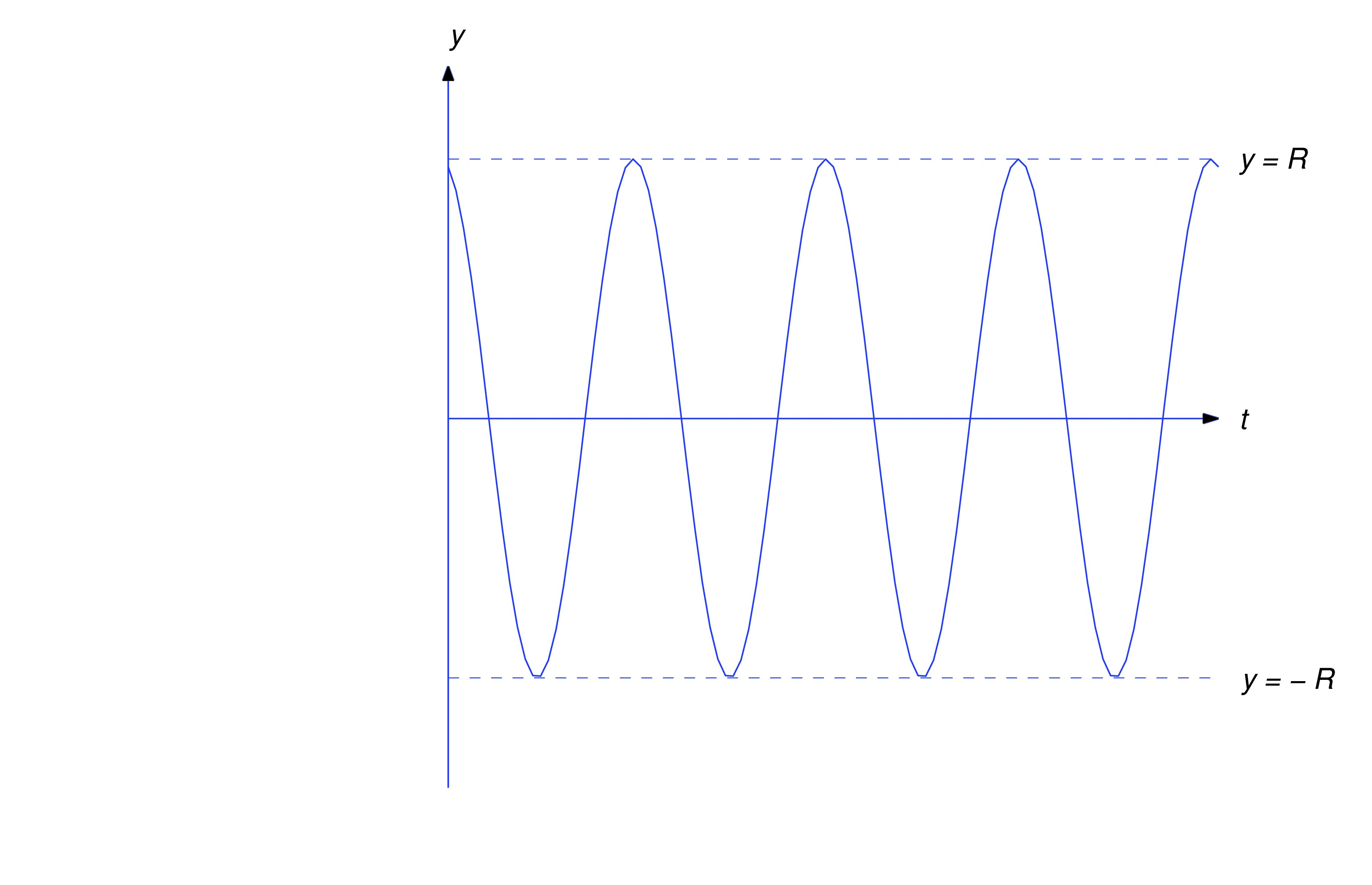
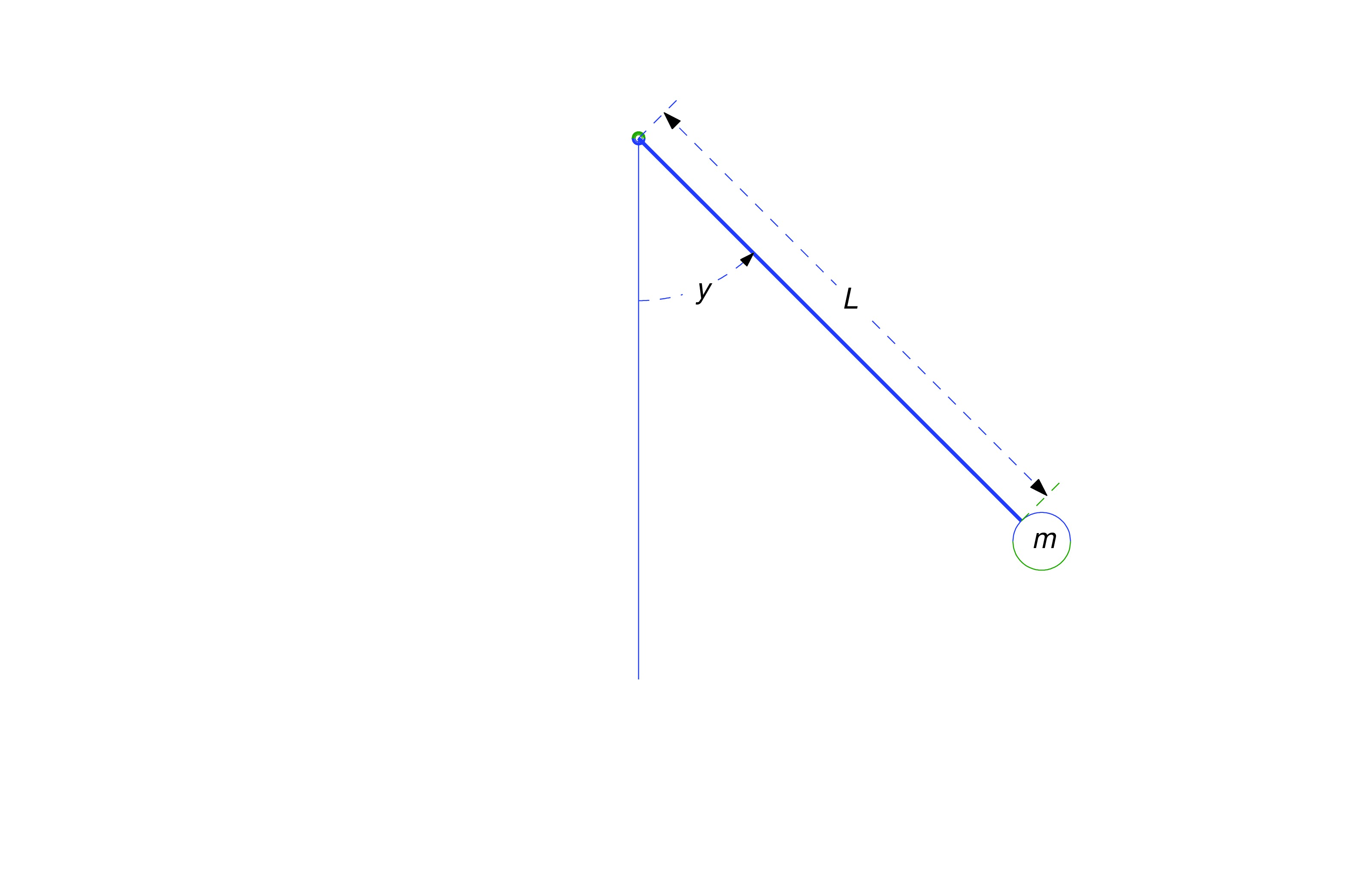
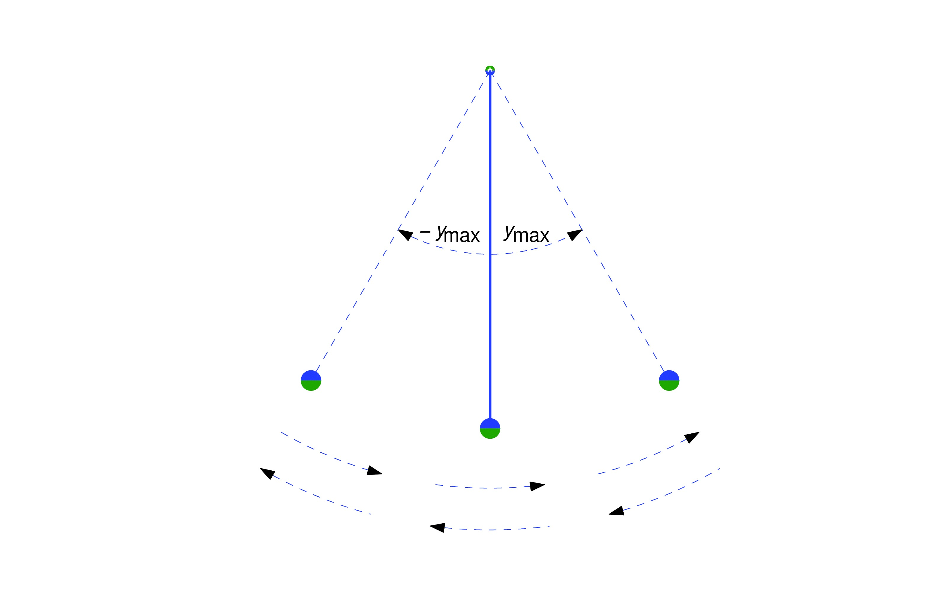
Let be the angle measured from the rest position (vertically downward) of the pendulum, as shown in the figure. Newton’s second law of motion says that the product of and the tangential acceleration equals the tangential component of the gravitational force. Therefore, or
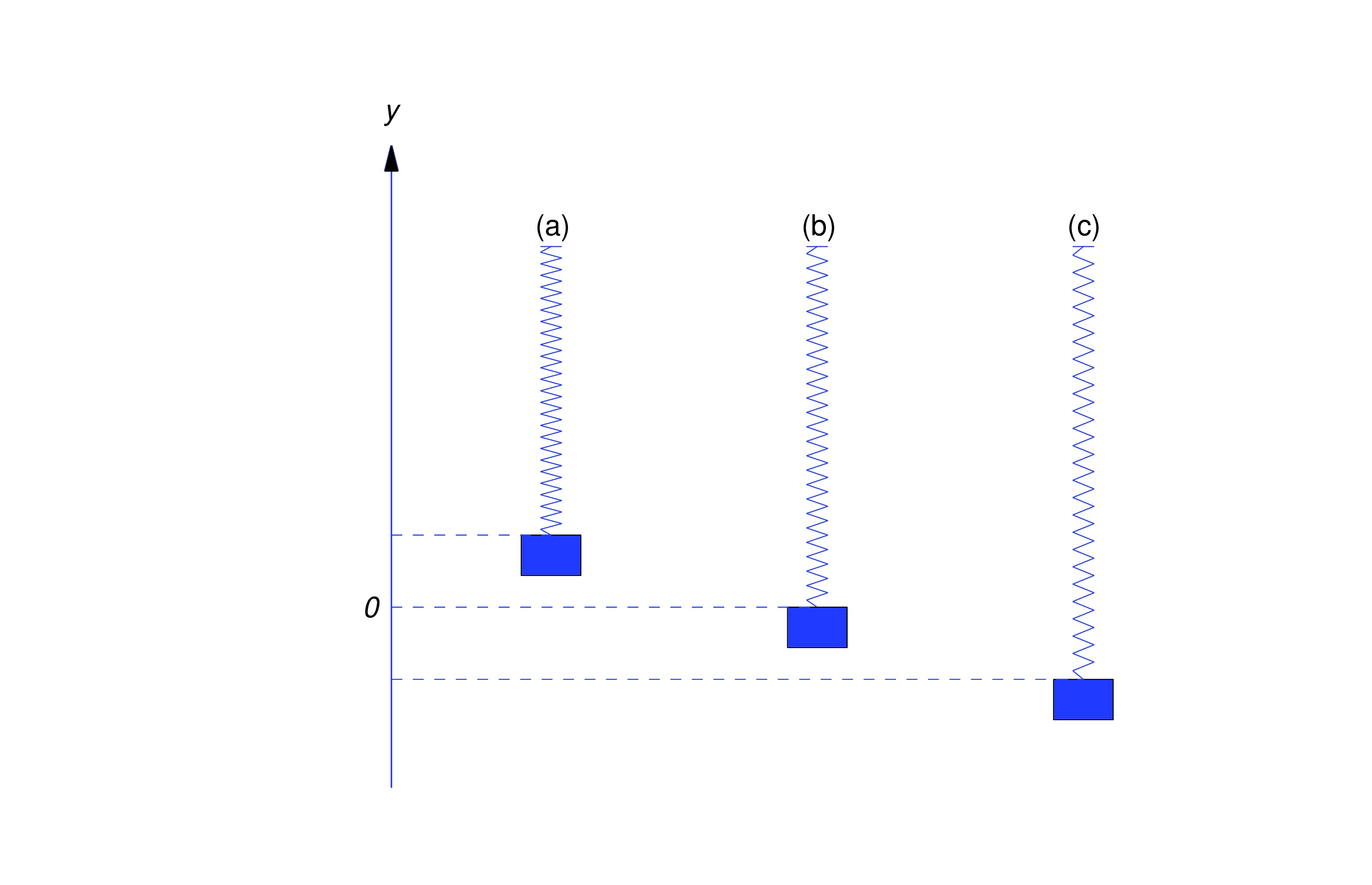
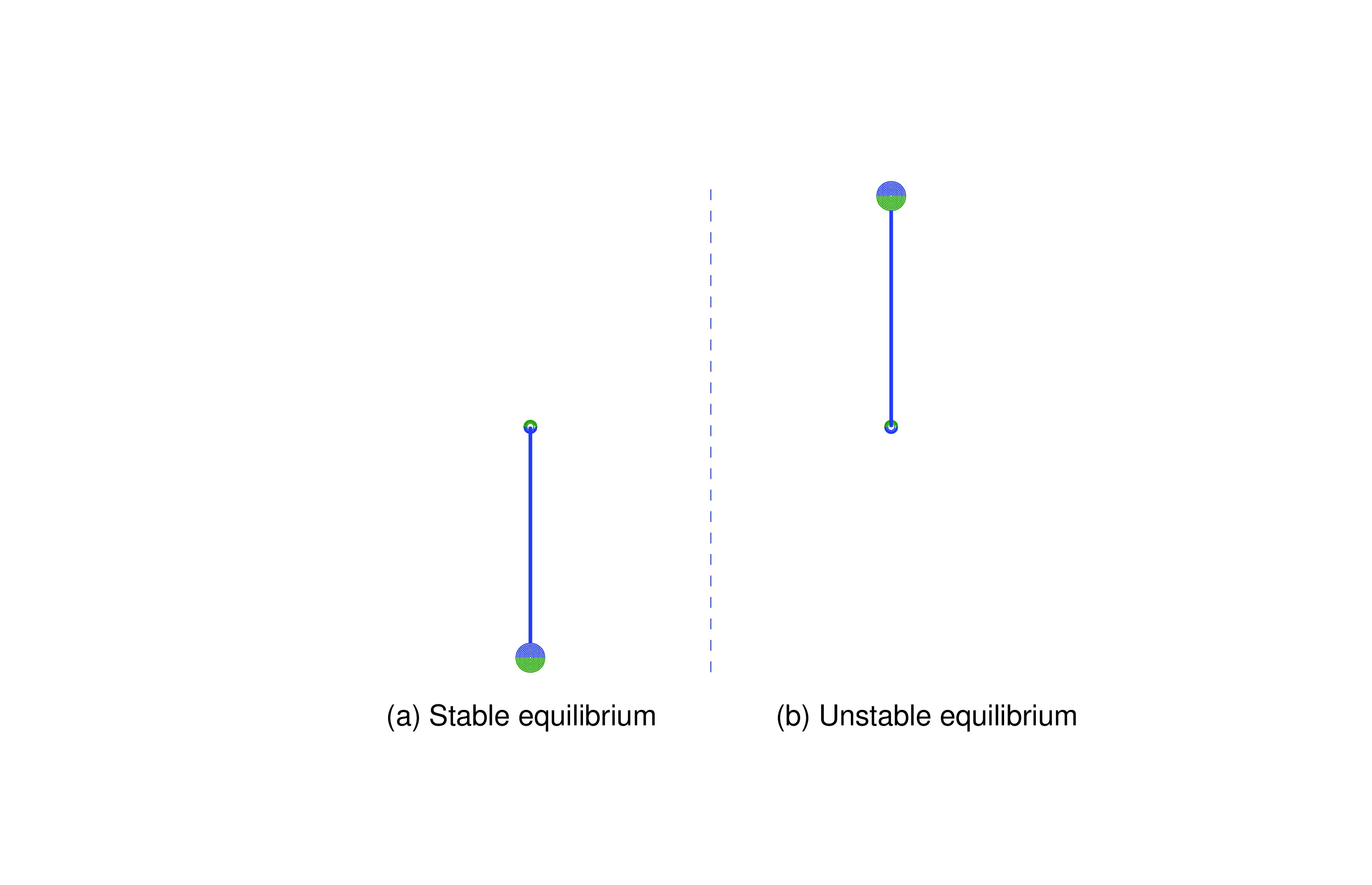
Since if is any integer, (eq:4.4.13) has infinitely many equilibria . If is even, the mass is directly below the axle, as shown in part (a) of the figure, and gravity opposes any deviation from the equilibrium. However, if is odd, the mass is directly above the axle, as shown in part (b), and gravity increases any deviation from the equilibrium. Therefore we conclude on physical grounds that is stable and is unstable.
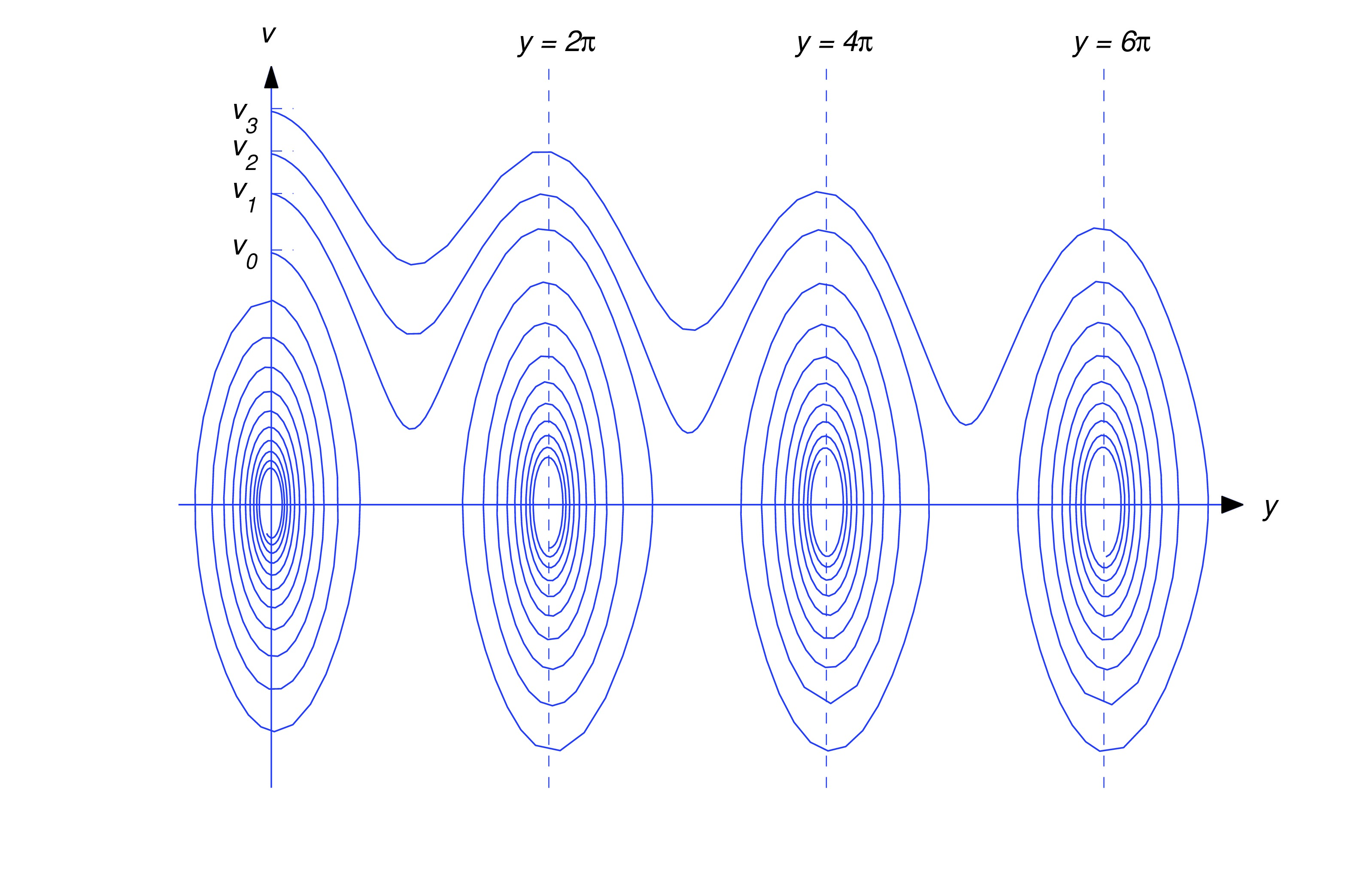
The phase plane equivalent of (eq:4.4.13) is where is the angular velocity of the pendulum. Integrating this yields
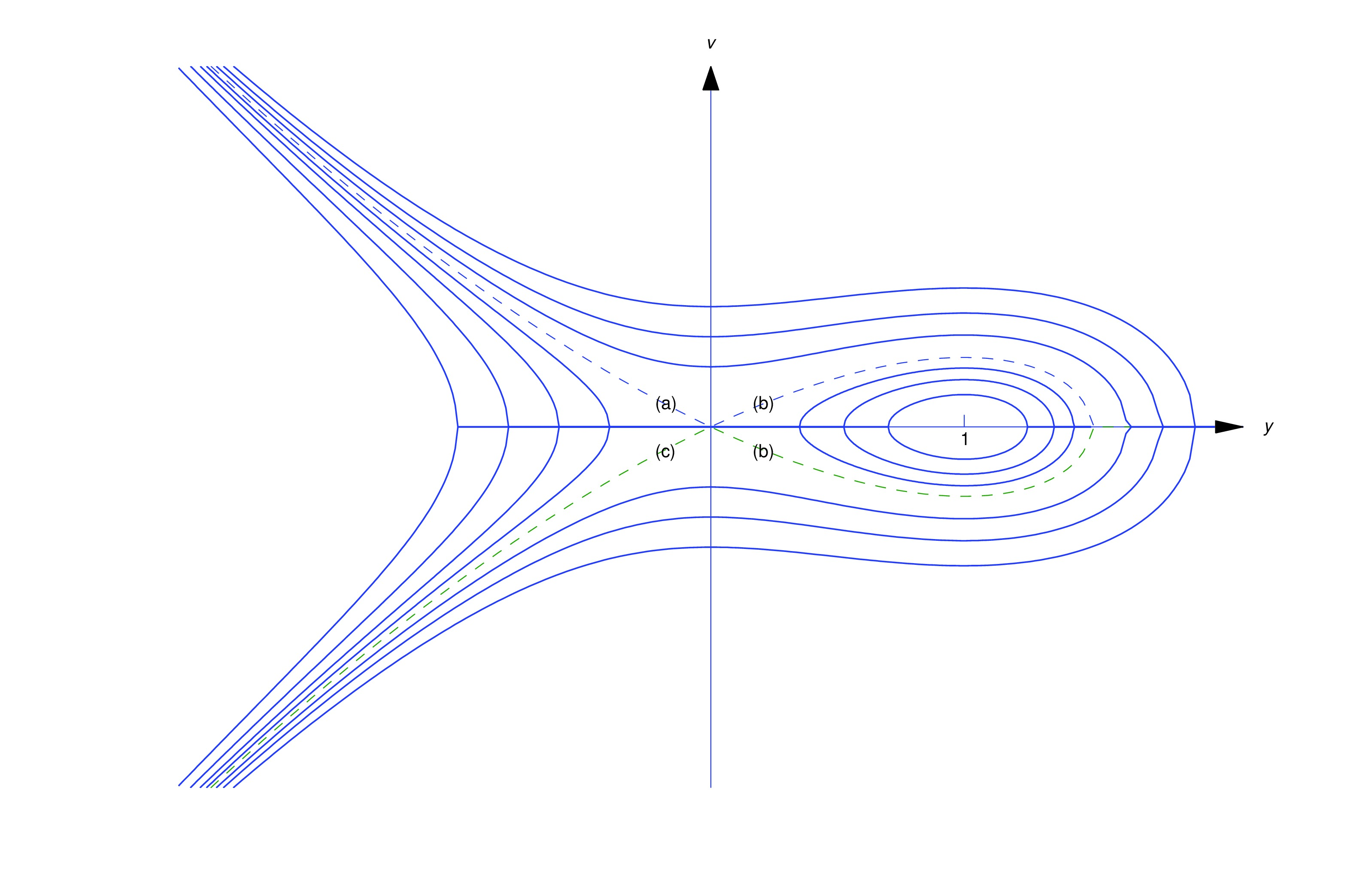
If when , then so (eq:4.4.14) becomes which is equivalent to whereThe curves defined by (eq:4.4.15) are the trajectories of (eq:4.4.13). They are periodic with period in , which isn’t surprising, since if is a solution of (eq:4.4.13) then so is for any integer . The figure below shows trajectories over the interval .
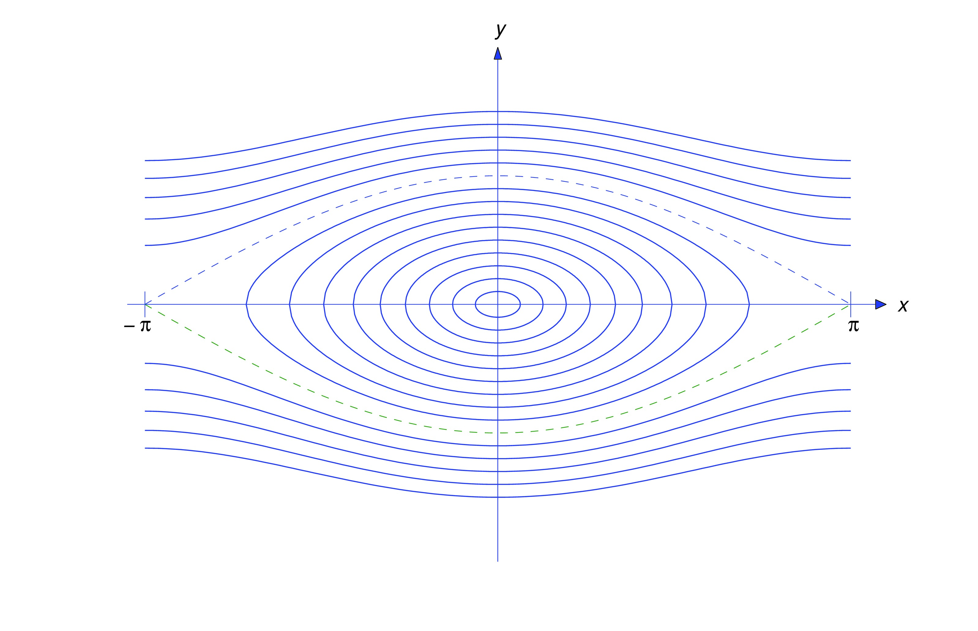
From (eq:4.4.15), you can see that if then is nonzero for all , which means that the object whirls in the same direction forever, as below.
In the first figure, the trajectories associated with this whirling motion are above the upper dashed curve and below the lower dashed curve. You can also see from (eq:4.4.15) that if ,then when , where In this case the pendulum oscillates periodically between and , as shown below.
The trajectories associated with this kind of motion are the ovals between the dashed curves in the first figure. It can be shown that the period of the oscillation is
Although this integral can’t be evaluated in terms of familiar elementary functions, you can see that it’s finite if .The dashed curves in the first figure contain four trajectories. The critical points and are the trajectories of the unstable equilibrium solutions . The upper dashed curve connecting (but not including) them is obtained from initial conditions of the form . If is any solution with this trajectory then The lower dashed curve connecting (but not including) them is obtained from initial conditions of the form . If is any solution with this trajectory then Consistent with this, the integral (eq:4.4.16) diverges to if .
Since the dashed curves separate trajectories of whirling solutions from trajectories of oscillating solutions, each of these curves is called a separatrix.
In general, if (eq:4.4.7) has both stable and unstable equilibria then the separatrices are the curves given by (eq:4.4.8) that pass through unstable critical points. Thus, if is an unstable critical point, then
defines a separatrix passing through .
Stability and Instability Conditions for
It can be shown that an equilibrium of an undamped equation
is stable if there’s an open interval containing such that If we regard as a force acting on a unit mass, (eq:4.4.19) means that the force resists all sufficiently small displacements from .We’ve already seen examples illustrating this principle. The equation (eq:4.4.9) for the undamped spring-mass system is of the form (eq:4.4.18) with , which has only the stable equilibrium . In this case (eq:4.4.19) holds with and . The equation (eq:4.4.13) for the undamped pendulum is of the form (eq:4.4.18) with . We’ve seen that is a stable equilibrium if is an integer. In this case and
It can also be shown that is unstable if there’s a such that
or an such that If we regard as a force acting on a unit mass, (eq:4.4.20) means that the force tends to increase all sufficiently small positive displacements from , while (eq:4.4.21) means that the force tends to increase the magnitude of all sufficiently small negative displacements from .The undamped pendulum also illustrates this principle. We’ve seen that is an unstable equilibrium if is an integer. In this case so (eq:4.4.20) holds with , and so (eq:4.4.21) holds with .
The phase plane equivalent of (eq:4.4.22) is the separable equation Integrating yields which we rewrite as
after renaming the constant of integration. These are the trajectories of (eq:4.4.22). If is any solution of (eq:4.4.22), the point moves along the trajectory of in the direction of increasing in the upper half plane (), or in the direction of decreasing in the lower half plane ().The figure below shows typical trajectories.
The dashed curve through the critical point , obtained by setting in (eq:4.4.23), separates the - plane into regions that contain different kinds of trajectories; again, we call this curve a separatrix. Trajectories in the region bounded by the closed loop labeled (b) are closed curves, so solutions associated with them are periodic. Solutions associated with other trajectories are not periodic. If is any such solution with trajectory not on the separatrix, then
The separatrix contains four trajectories of (eq:4.4.22). One is the point , the trajectory of the equilibrium . Since distinct trajectories can’t intersect, the segments of the separatrix marked (a), (b), and (c) – which don’t include – are distinct trajectories, none of which can be traversed in finite time. Solutions with these trajectories have the following asymptotic behavior:
The Damped Case
The phase plane equivalent of the damped autonomous equation
is This equation isn’t separable, so we can’t solve it for in terms of , as we did in the undamped case, and conservation of energy doesn’t hold. (For example, energy expended in overcoming friction is lost.) However, we can study the qualitative behavior of its solutions by rewriting it as and considering the direction fields for this equation. In the following examples we’ll also be showing computer generated trajectories of this equation, obtained by numerical methods. The exercises call for similar computations. The methods discussed in Trench 3.1–3.3 are not suitable for this task, since in (eq:4.4.25) is undefined on the axis of the Poincaré phase plane. Therefore we’re forced to apply numerical methods briefly discussed in Trench 10.1 to the systemIn the text we’ll confine ourselves to the case where is constant, so (eq:4.4.24) and (eq:4.4.25) reduce to
and (We’ll consider more general equations in the exercises.) The constant is called the damping constant. In situations where (eq:4.4.26) is the equation of motion of an object, is positive; however, there are situations where may be negative.The Damped Spring-Mass System
Earlier we considered the spring - mass system under the assumption that the only forces acting on the object were gravity and the spring’s resistance to changes in its length. Now we’ll assume that some mechanism (for example, friction in the spring or atmospheric resistance) opposes the motion of the object with a force proportional to its velocity. In Trench 6.1 it will be shown that in this case Newton’s second law of motion implies that
where is the damping constant. Again, this equation can be solved easily by a method that we’ll study in Trench 5.2, but that method isn’t available here. Instead, we’ll consider its phase plane equivalent, which can be written in the form (eq:4.4.25) as (A minor note: the in (eq:4.4.26) actually corresponds to in this equation.) The figure below shows a typical direction field for an equation of this form.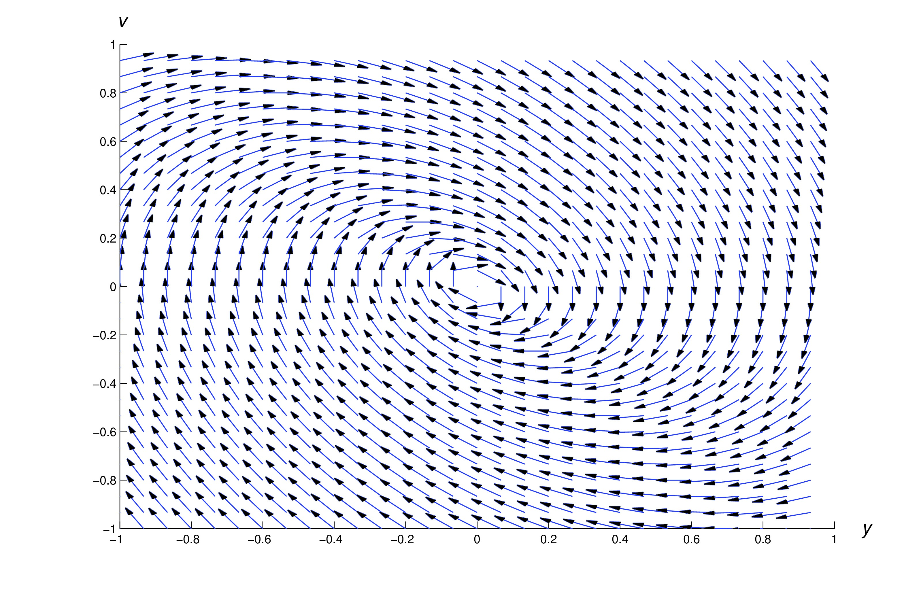
Recalling that motion along a trajectory must be in the direction of increasing in the upper half plane () and in the direction of decreasing in the lower half plane (), you can infer that all trajectories approach the origin in clockwise fashion. To confirm this, the following figure shows the same direction field with some trajectories filled in.
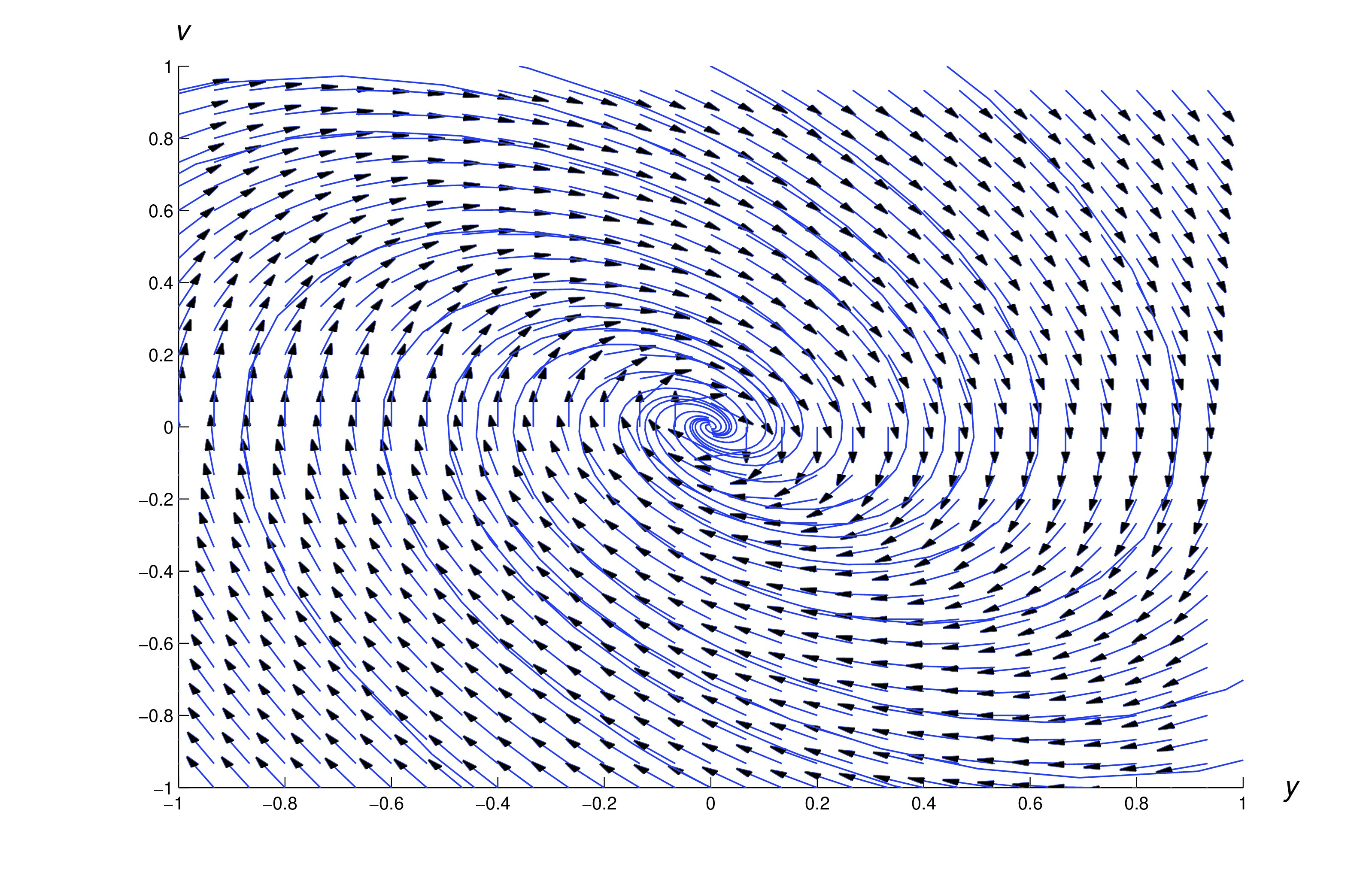
All the trajectories shown there correspond to solutions of the initial value problem where thus, if there were no damping (), all the solutions would have the same dashed elliptic trajectory, shown below.
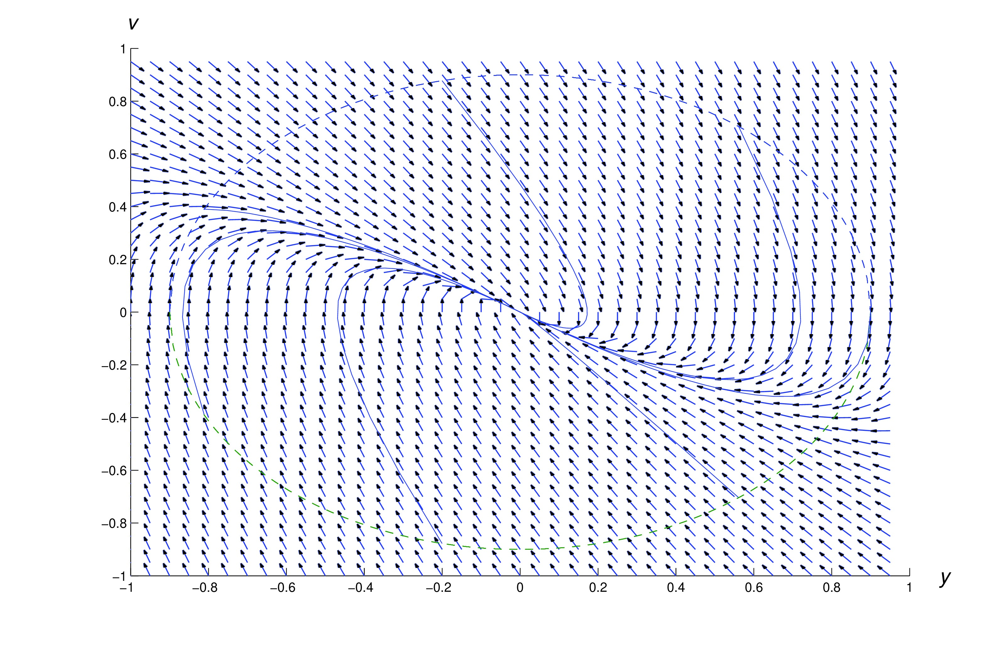
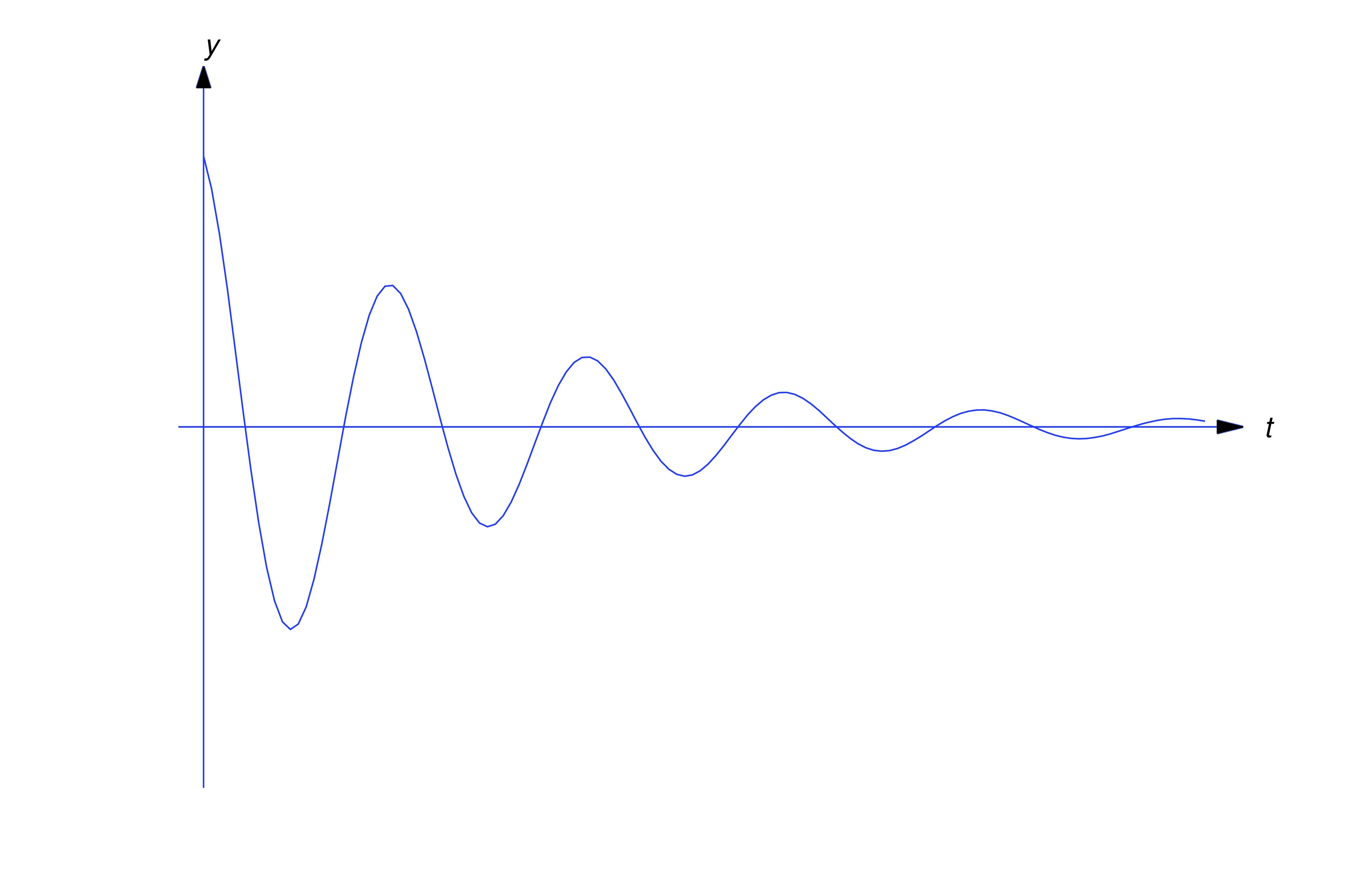
Solutions corresponding to the trajectories in this figure cross the -axis infinitely many times.
The corresponding solutions, shown below, are said to be oscillatory
It is shown in Trench 6.2 that there’s a number such that if then all solutions of (eq:4.4.27) are oscillatory, while if , no solutions of (eq:4.4.27) have this property. (In fact, no solution not identically zero can have more than two zeros in this case.) The following figure shows a direction field and some integral curves for (eq:4.4.28) in this case.
Text Source
Trench, William F., ”Elementary Differential Equations” (2013). Faculty Authored and Edited Books & CDs. 8. (CC-BY-NC-SA)