We study an existence and uniqueness theorem for a first-order initial value problem. We do not attempt the proof, as it is beyond the scope of this book.
Existence and Uniqueness of Solutions of Nonlinear Equations
Although there are methods for solving some nonlinear equations, it’s impossible to find useful formulas for the solutions of most. Whether we’re looking for exact solutions or numerical approximations, it’s useful to know conditions that imply the existence and uniqueness of solutions of initial value problems for nonlinear equations. In this section we state such a condition and illustrate it with examples.
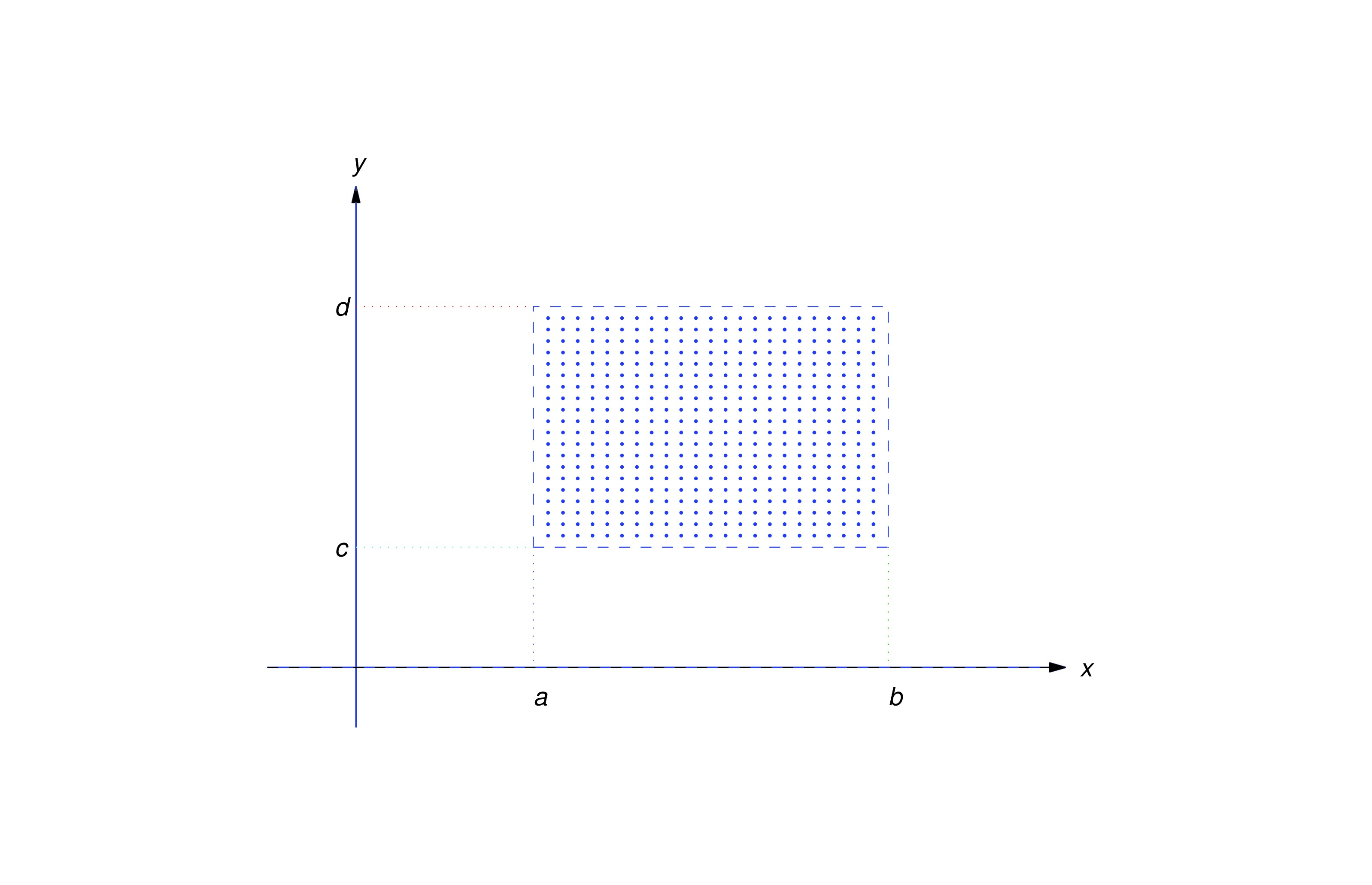
Some terminology: an open rectangle is a set of points such that (see figure above). We’ll denote this set by . “Open” means that the boundary rectangle (indicated by the dashed lines in the figure) isn’t included in .
The next theorem gives sufficient conditions for existence and uniqueness of solutions of initial value problems for first order nonlinear differential equations. We omit the proof, which is beyond the scope of this book.
- (a)
- If is continuous on an open rectangle that contains then the initial value problem has at least one solution on some open subinterval of that contains
- (b)
- If both and are continuous on then (eq:2.3.1) has a unique solution on some open subinterval of that contains .
It’s important to understand exactly what Theorem thmtype:2.3.1 says.
- Part thmtype:2.3.1a is an existence theorem. It guarantees that a solution exists on some open interval that contains , but provides no information on how to find the solution, or to determine the open interval on which it exists. Moreover, part thmtype:2.3.1a provides no information on the number of solutions that (eq:2.3.1) may have. It leaves open the possibility that (eq:2.3.1) may have two or more solutions that differ for values of arbitrarily close to . We will see in Example example:2.3.6 that this can happen.
- Part thmtype:2.3.1b is a uniqueness theorem. It guarantees that (eq:2.3.1) has a unique solution on some open interval (a,b) that contains . However, if , (eq:2.3.1) may have more than one solution on a larger interval that contains . For example, it may happen that and all solutions have the same values on , but two solutions and are defined on some interval with , and have different values for ; thus, the graphs of the and “branch off” in different directions at . (See Example example:2.3.7 and the figure below it. In this case, continuity implies that (call their common value ), and and are both solutions of the initial value problem that differ on every open interval that contains . Therefore or must have a discontinuity at some point in each open rectangle that contains , since if this were not so, (eq:2.3.2) would have a unique solution on some open interval that contains . We leave it to you to give a similar analysis of the case where .
- (a)
- For what points does Theorem thmtype:2.3.1, part thmtype:2.3.1a imply that (eq:2.3.8) has a solution?
- (b)
- For what points does Theorem thmtype:2.3.1, part thmtype:2.3.1b imply that (eq:2.3.8) has a unique solution on some open interval that contains ?
eq:2.3.8b Here is continuous for all with . Therefore, if there’s an open rectangle on which both and are continuous, and Theorem thmtype:2.3.1 implies that (eq:2.3.8) has a unique solution on some open interval that contains .
If then is undefined, and therefore discontinuous; hence, Theorem thmtype:2.3.1 does not apply to (eq:2.3.8) if .
Now suppose is a solution of (eq:2.3.10) that isn’t identically zero. Separating variables in (eq:2.3.10) yields on any open interval where has no zeros. Integrating this and rewriting the arbitrary constant as yields Therefore
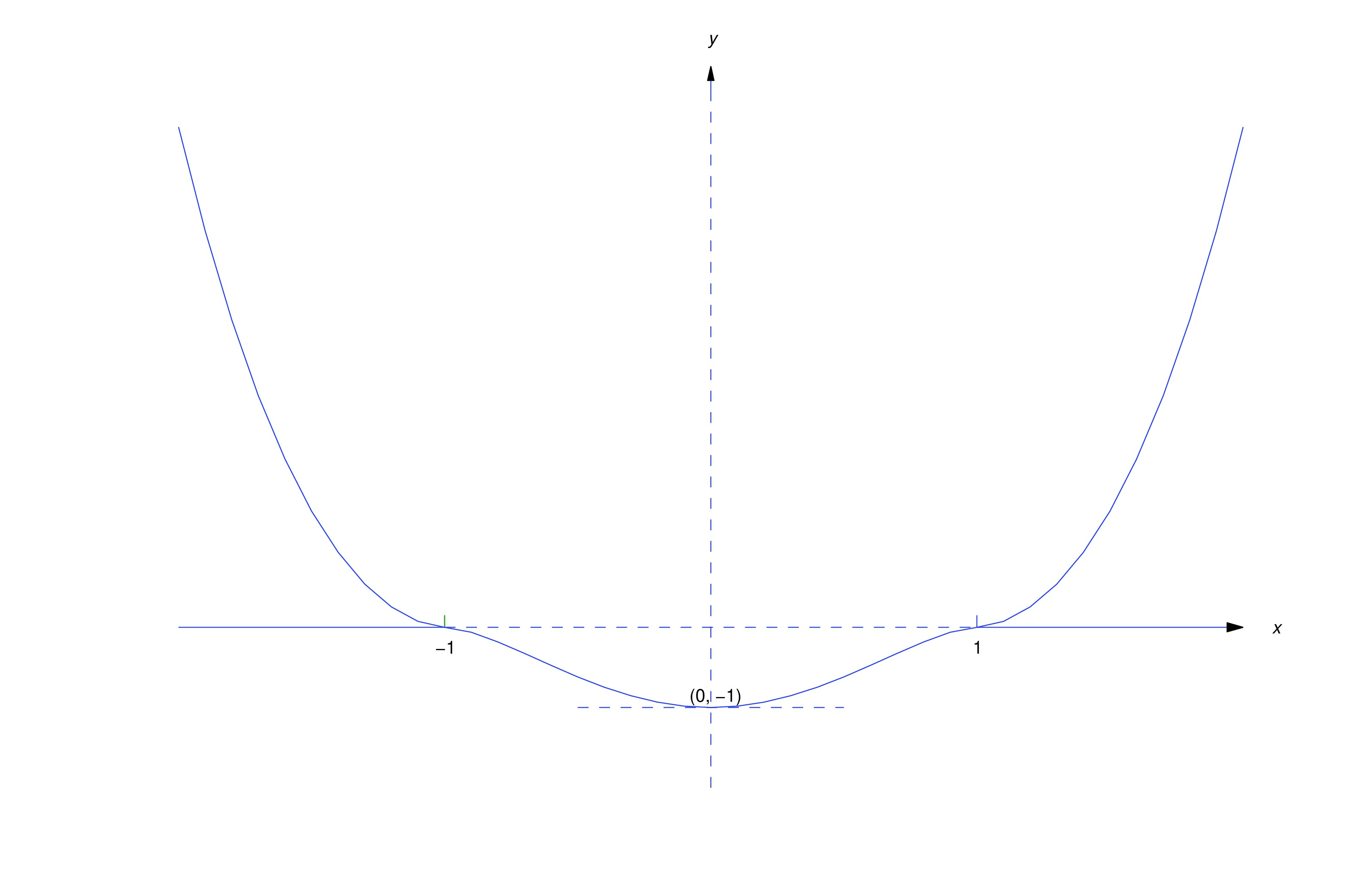
Since we divided by to separate variables in (eq:2.3.10), our derivation of (eq:2.3.11) is legitimate only on open intervals where has no zeros. However, (eq:2.3.11) actually defines for all , and differentiating (eq:2.3.11) shows that Therefore (eq:2.3.11) satisfies (eq:2.3.10) on even if , so that . In particular, taking in (eq:2.3.11) yields as a second solution of (eq:2.3.9). Both solutions are defined on , and they differ on every open interval that contains (see the figure below). In fact, there are four distinct solutions of (eq:2.3.9) defined on that differ from each other on every open interval that contains . Can you identify the other two?

Text Source
Trench, William F., ”Elementary Differential Equations” (2013). Faculty Authored and Edited Books & CDs. 8. (CC-BY-NC-SA)