We solve a separable differential equation and describe a few of its many applications.
Exponential Growth and Decay
Since the applications in this section deal with functions of time, we’ll denote the independent variable by . If is a function of , will denote the derivative of with respect to ; thus,
Exponential Growth and Decay
One of the most common mathematical models for a physical process is the exponential model, where it’s assumed that the rate of change of a quantity is proportional to ; thus
where is the constant of proportionality.The general solution of (eq:4.1.1) is and the solution of the initial value problem is
Since the solutions of are exponential functions, we say that a quantity that satisfies this equation grows exponentially if , or decays exponentially if (see figure below).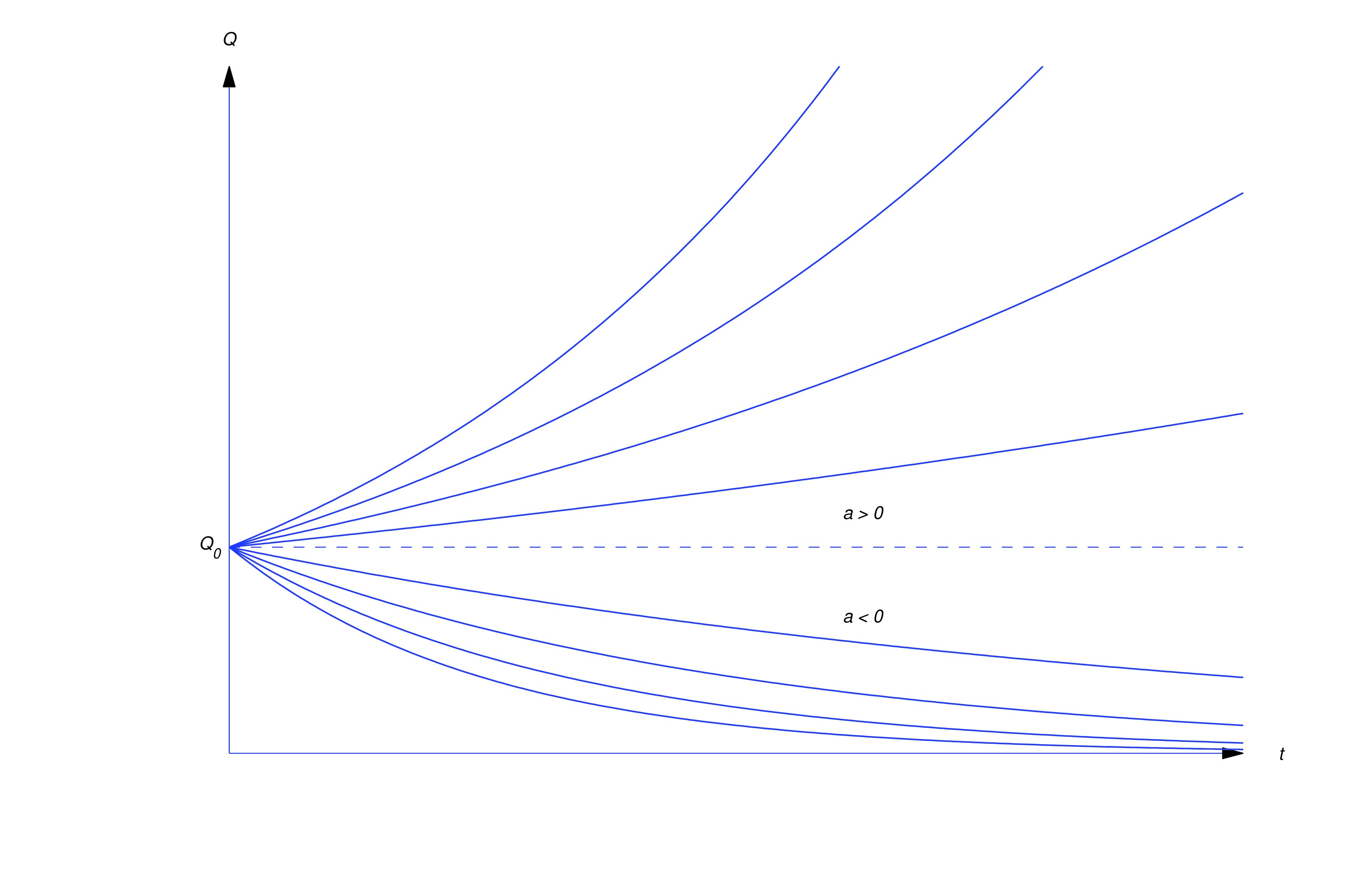
Radioactive Decay
Experimental evidence shows that radioactive material decays at a rate proportional to the mass of the material present. According to this model the mass of a radioactive material present at time satisfies (eq:4.1.1), where is a negative constant whose value for any given material must be determined by experimental observation. For simplicity, we’ll replace the negative constant by , where is a positive number that we’ll call the decay constant of the material. Thus, (eq:4.1.1) becomes If the mass of the material present at is , the mass present at time is the solution of From (eq:4.1.2) with , the solution of this initial value problem is
The half–life of a radioactive material is defined to be the time required for half of its mass to decay; that is, if , then
From (eq:4.1.3) with , (eq:4.1.4) is equivalent to so Taking logarithms yields so the half-life is (see figure below). The half-life is independent of and , since it’s determined by the properties of material, not by the amount of the material present at any particular time.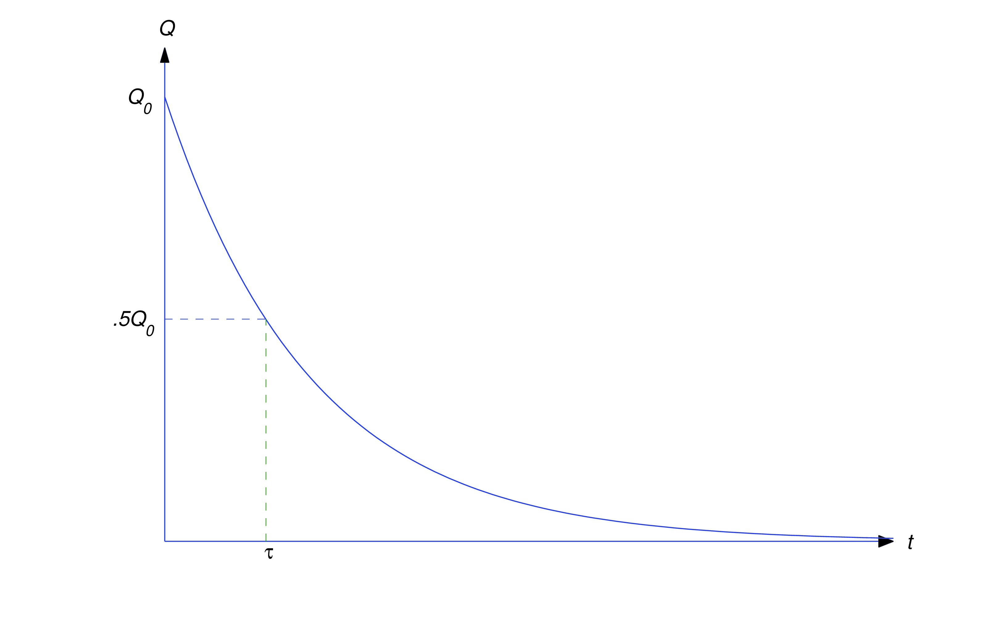
- (a)
- If its mass is now 4 g (grams), how much will be left 810 years from now?
- (b)
- Find the time when 1.5 g of the substance remain.
item:4.1.1b Setting in (eq:4.1.7) and requiring that yields Dividing by 4 and taking logarithms yields Since ,
Interest Compounded Continuously
Suppose we deposit an amount of money in an interest-bearing account and make no further deposits or withdrawals for years, during which the account bears interest at a constant annual rate . To calculate the value of the account at the end of years, we need one more piece of information: how the interest is added to the account, or—as the bankers say—how it is compounded. If the interest is compounded annually, the value of the account is multiplied by at the end of each year. This means that after years the value of the account is If interest is compounded semiannually, the value of the account is multiplied by every 6 months. Since this occurs twice annually, the value of the account after years is In general, if interest is compounded times per year, the value of the account is multiplied times per year by ; therefore, the value of the account after years is
Thus, increasing the frequency of compounding increases the value of the account after a fixed period of time. The table below shows the effect of increasing the number of compoundings over years on an initial deposit of (dollars), at an annual interest rate of 6%.
You can see from the table above that the value of the account after 5 years is an increasing function of . Now suppose the maximum allowable rate of interest on savings accounts is restricted by law, but the number of times a bank can compound in a given time interval isn’t; then competing banks can attract savers by compounding often. The ultimate step in this direction is to compound continuously, by which we mean that in (eq:4.1.8). Since we know from calculus that this yields Observe that is the solution of the initial value problem that is, with continuous compounding the value of the account grows exponentially.
Mixed Growth and Decay
item:4.1.4b Since , , so from (eq:4.1.12) This limit depends only on and , and not on . We say that is the steady state value of . From (eq:4.1.12) we also see that approaches its steady state value from above if , or from below if . If , then remains constant (see figure below).

Carbon Dating
The fact that approaches a steady state value in the situation discussed in Example 4 underlies the method of carbon dating, devised by the American chemist and Nobel Prize Winner W.S. Libby.
Carbon 12 is stable, but carbon-14, which is produced by cosmic bombardment of nitrogen in the upper atmosphere, is radioactive with a half-life of about 5570 years. Libby assumed that the quantity of carbon-12 in the atmosphere has been constant throughout time, and that the quantity of radioactive carbon-14 achieved its steady state value long ago as a result of its creation and decomposition over millions of years. These assumptions led Libby to conclude that the ratio of carbon-14 to carbon-12 has been nearly constant for a long time. This constant, which we denote by , has been determined experimentally.
Living cells absorb both carbon-12 and carbon-14 in the proportion in which they are present in the environment. Therefore the ratio of carbon-14 to carbon-12 in a living cell is always . However, when the cell dies it ceases to absorb carbon, and the ratio of carbon-14 to carbon-12 decreases exponentially as the radioactive carbon-14 decays. This is the basis for the method of carbon dating, as illustrated in the next example.
A Savings Program
Mathematical models must be tested for validity by comparing predictions based on them with the actual outcome of experiments. Example 6 is unusual in that we can compute the exact value of the account at any specified time and compare it with the approximate value predicted by (eq:4.1.15) The following table gives a comparison for a ten year period. Each exact answer corresponds to the time of the year-end deposit, and each year is assumed to have exactly 52 weeks.
Text Source
Trench, William F., ”Elementary Differential Equations” (2013). Faculty Authored and Edited Books & CDs. 8. (CC-BY-NC-SA)