We explore direction fields (also called slope fields) for some examples of first order differential equations.
Direction Fields for First Order Equations
We cannot (yet!) solve the differential equation However, from the equation alone, we can deduce some facts about the solution. Recall that, geometrically speaking, the value of the first derivative of a function at a point is the slope of the tangent line to the graph of the function at that point. So, given a differential equation of the form
we can interpret the value as the slope of the tangent line to the graph of at the point . Thus, the differential equation tells us the slope of any solution passing through a given point. Consider the solution to the differential equation which passes through the point
. What is the slope of the tangent line to solution at The slope of at is .
Given a differential equation, say , we can pick points in the plane and compute what the slope of a solution at those points will be. Repeating this process, we can generate a slope field. The slope field for the differential equation looks like this:

Let’s be explicit:
A slope field, also called a direction field, is a graphical aid for
understanding a differential equation, formed by:
- Choosing a grid of points.
- At each point, computing the slope given by the differential equation, using the and -values of the point.
- At each point, drawing a short line segment with that slope.
Here is the slope field for the differential equation , with a few solutions of the differential equation also graphed.

Each of the many solutions to the differential equation is determined by initial conditions. The following interactive allows you to input the initial condition in the dialog box. The output displays the slope field together with point and the solution that satisfies the initial condition.


Given a differential equation such as , it is easy to find an explicit solution to the equation. (You may want to verify that functions of the form are solutions.) However, it’s impossible to find explicit formulas for solutions of some differential equations. Even if there are such formulas, they may be so complicated that they’re useless. In this case we may resort to graphical or numerical methods to get some idea of how the solutions of the given equation behave. Slope fields offer us one such method.
As we will see, the combination of direction fields and integral curves gives useful insights into the behavior of the solutions of the differential equation even if we can’t obtain exact solutions.
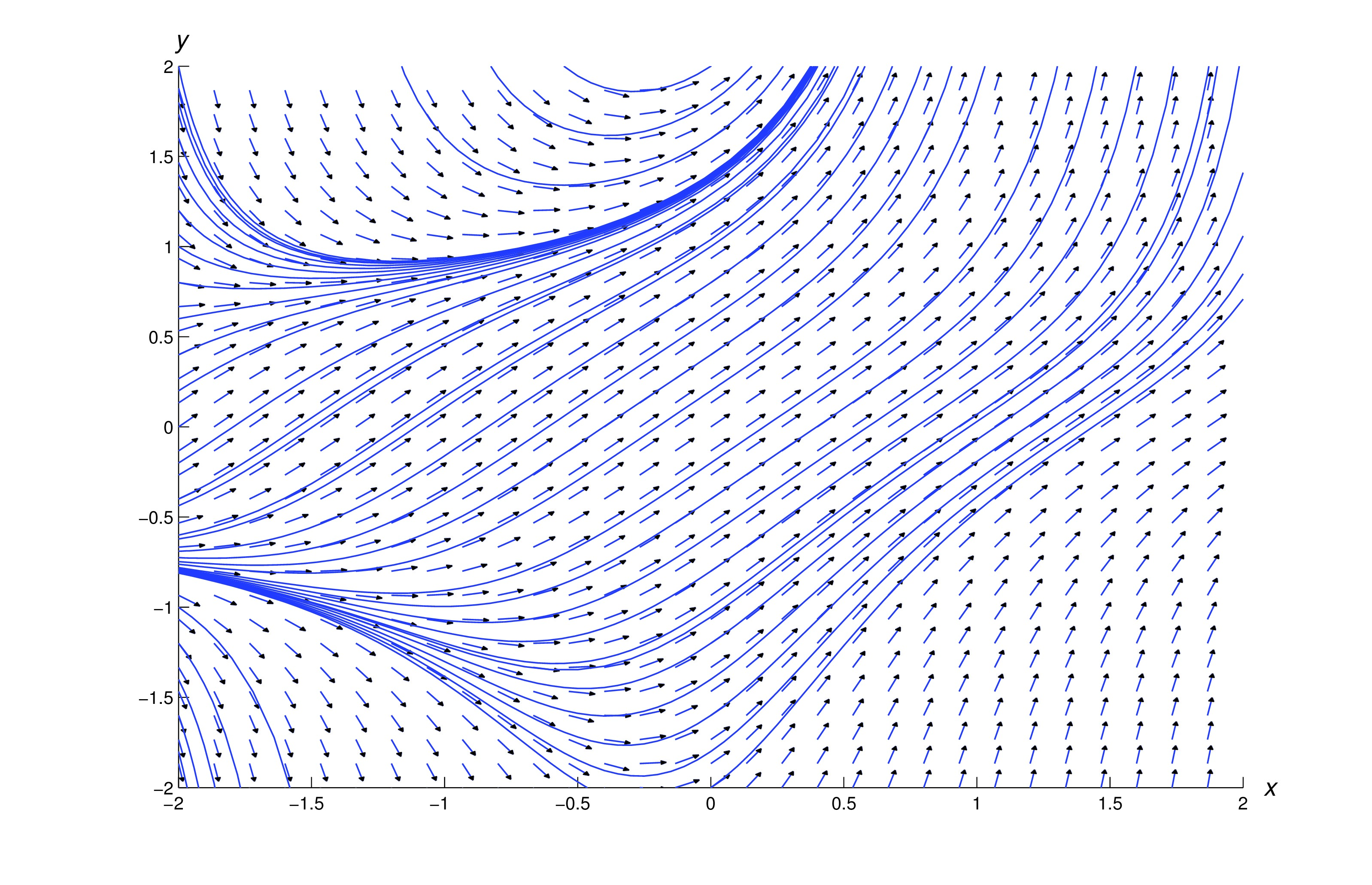
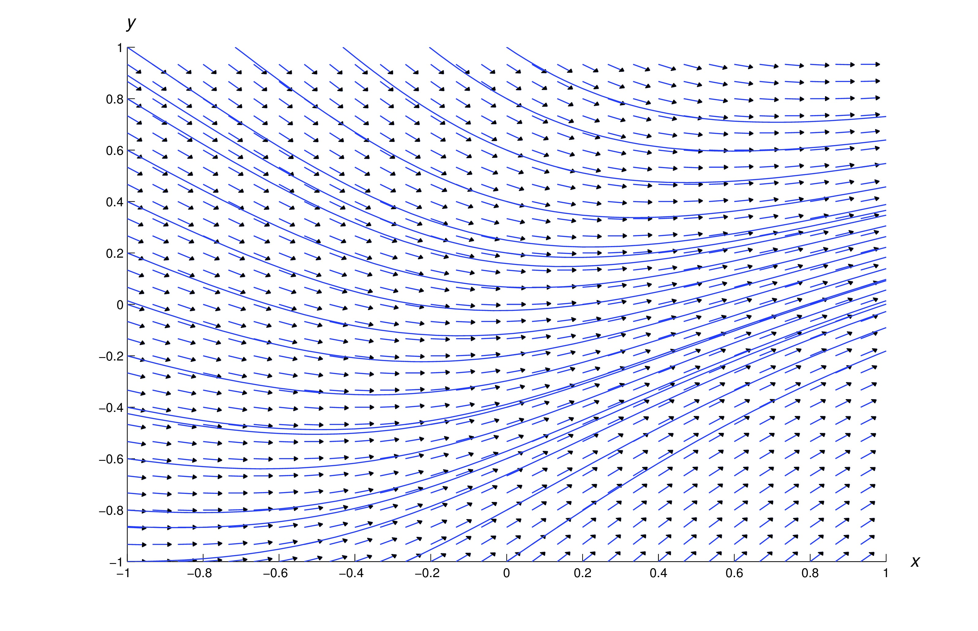
We’ll study numerical methods for solving a single first order equation (eq:1.3.1) in Trench 3.1 - Trench 3.3. These methods can be used to plot solution curves of (eq:1.3.1) in a rectangular region if is continuous on . The figures in the three examples below show direction fields and solution curves for several differential equations of the form (eq:1.3.1) with continuous for all .
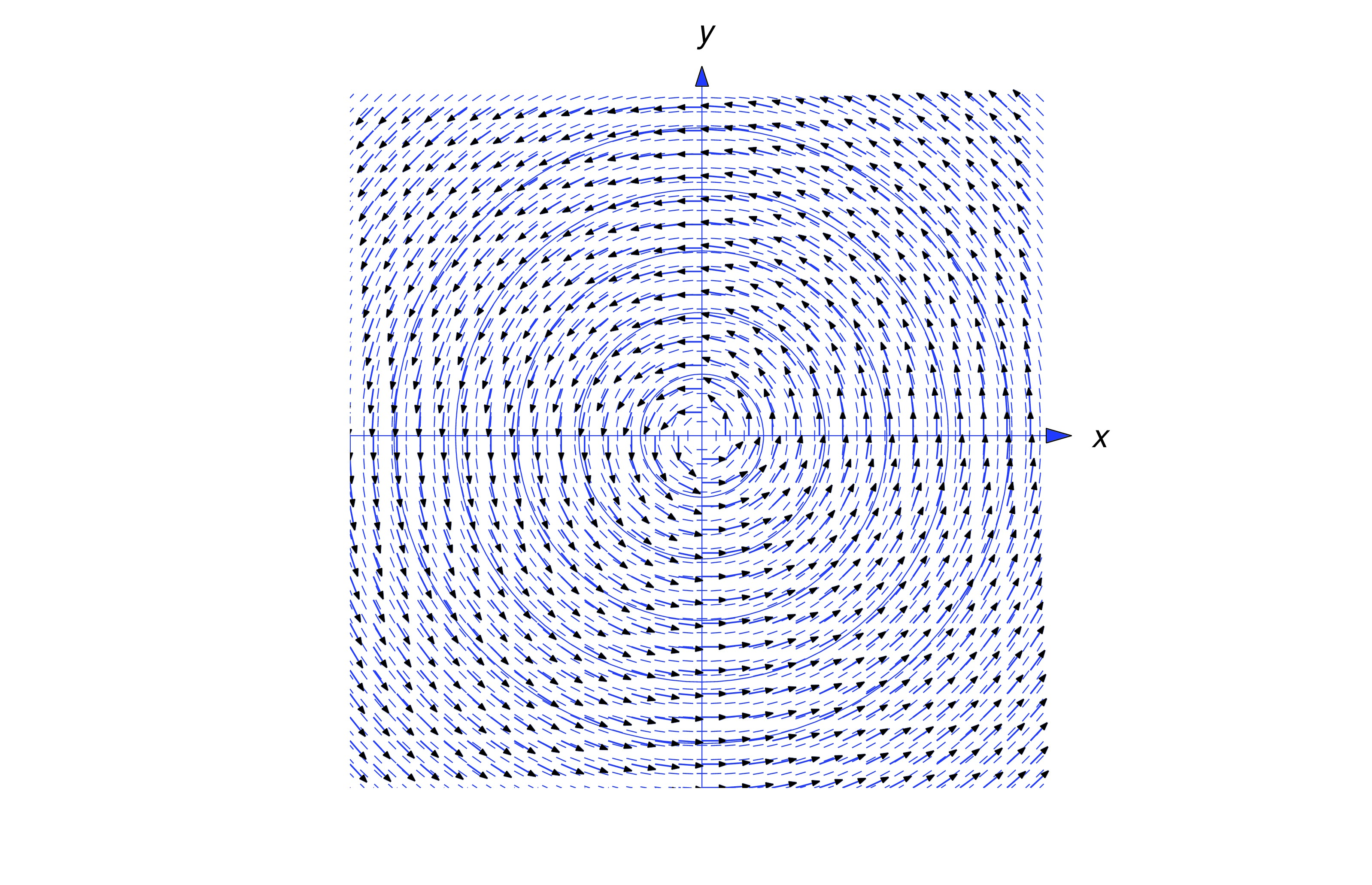
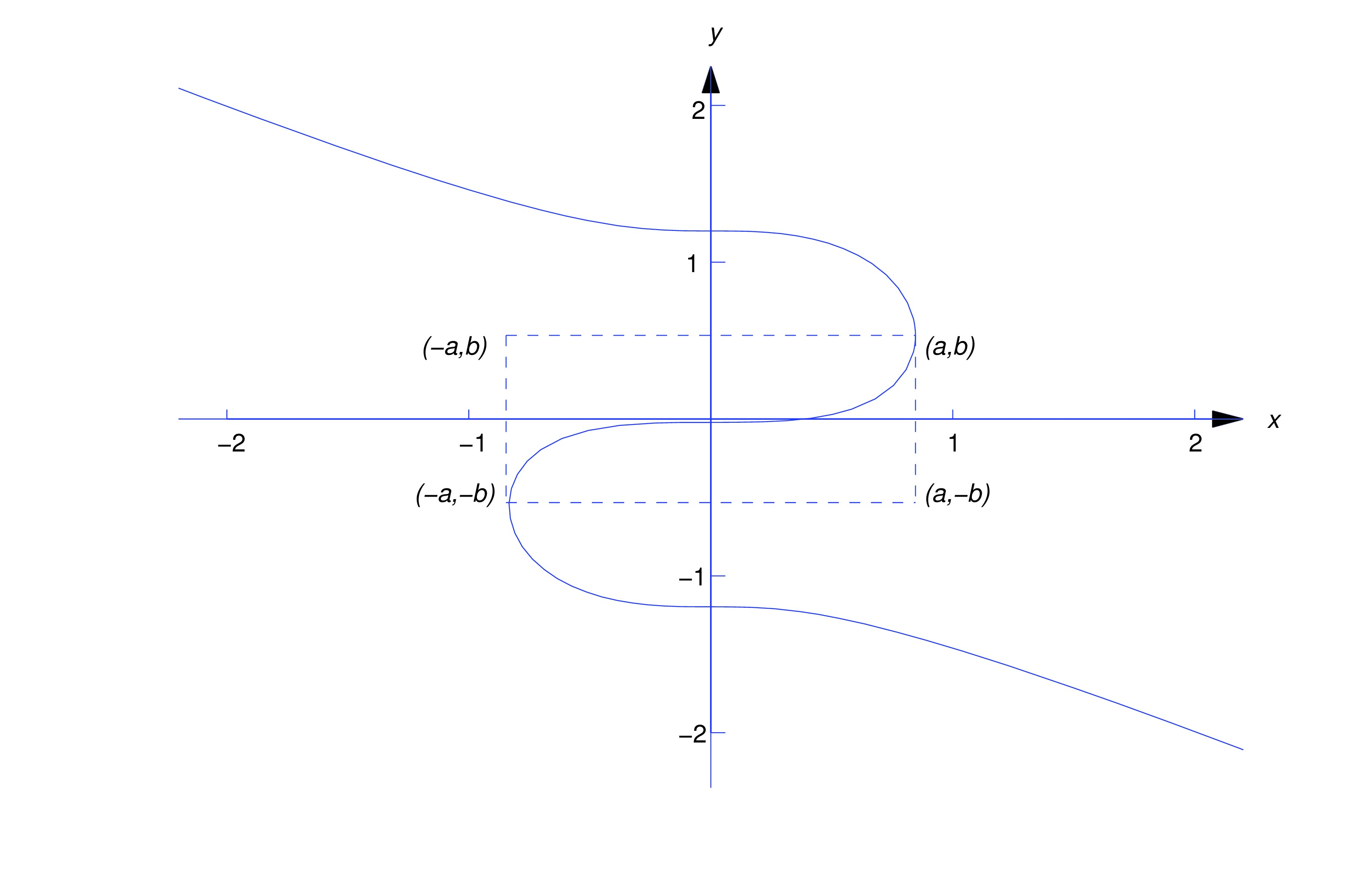
The methods of Trench 3.1 - Trench 3.3 won’t work for the equation if contains part of the -axis, since is undefined when . Similarly, they won’t work for the equation if contains any part of the unit circle , because the right side of (eq:1.3.3) is undefined if . However, (eq:1.3.2) and (eq:1.3.3) can written as where and are continuous on any rectangle . Because of this, some differential equation software is based on numerically solving pairs of equations of the form where and are regarded as functions of a parameter . If and satisfy these equations, then so satisfies (eq:1.3.4).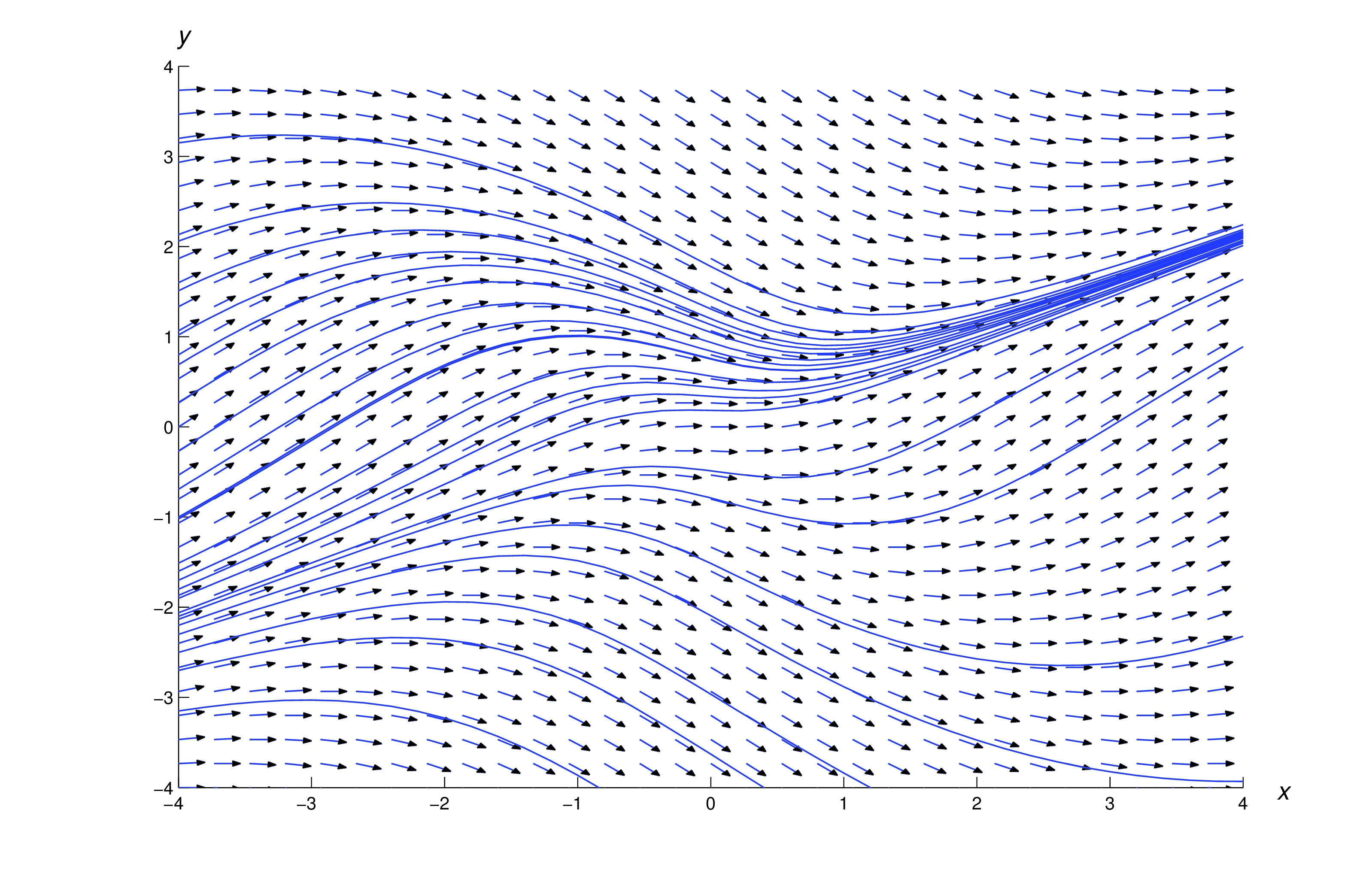
Eqns. (eq:1.3.2) and (eq:1.3.3) can be reformulated as in (eq:1.3.4) with and respectively.
The figure below shows a direction field and some integral curves for . As we saw in Example example:1.2.1, the integral curves of (eq:1.3.2) are circles centered at the origin.
The figure below shows a direction field and some integral curves for .
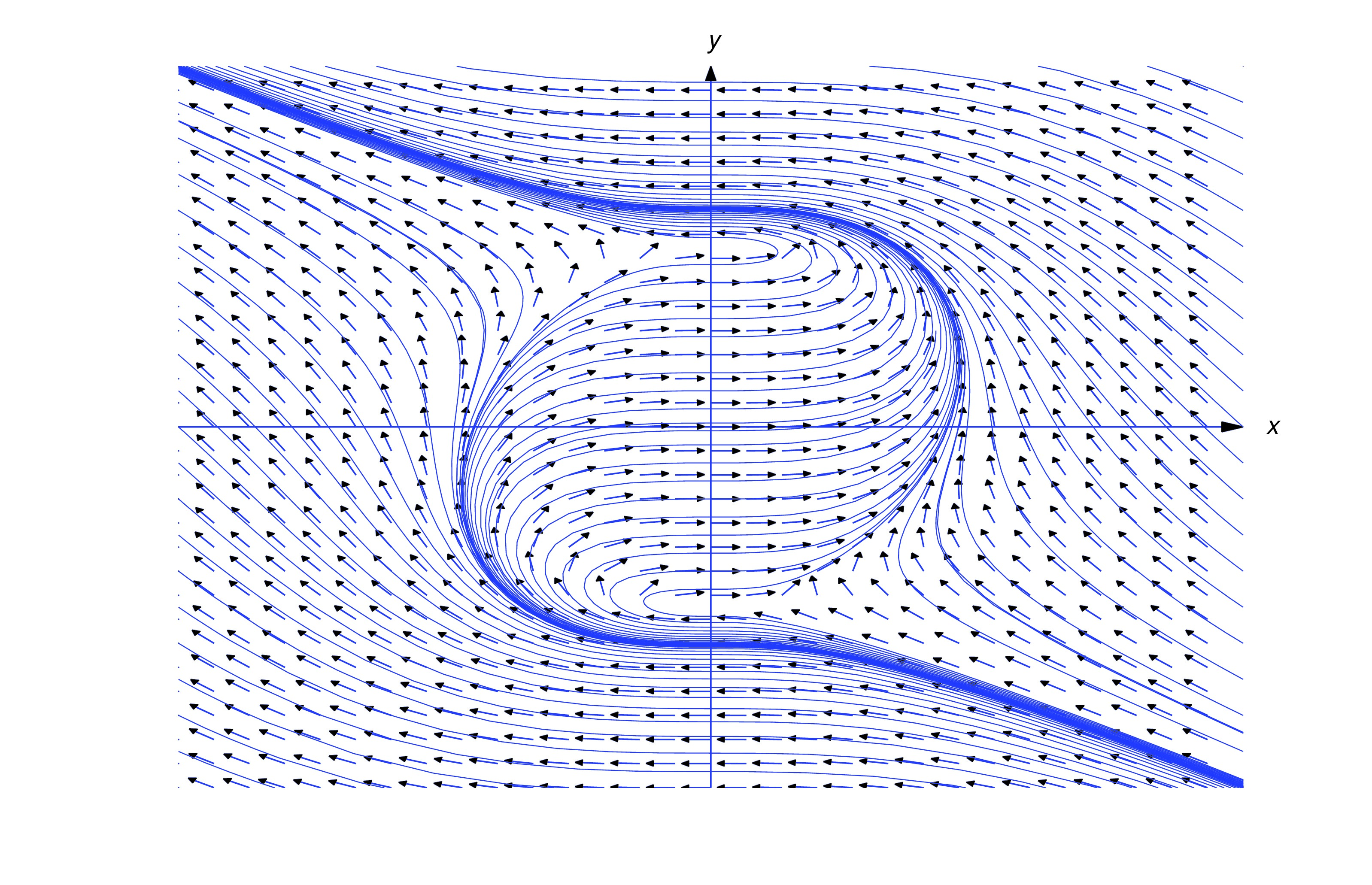
Even if is continuous and otherwise “nice” throughout , your software may require you to reformulate the equation as which is of the form (eq:1.3.5) with and .
As you study from this book, you’ll often be asked to use computer software and graphics. Often you may not completely understand how the software does what it does. This is similar to the situation most people are in when they drive automobiles or watch television, and it doesn’t decrease the value of using modern technology as an aid to learning. Just be careful that you use the technology as a supplement to thought rather than a substitute for it.
Text Source
MOOCulus, Numerical Methods (CC-BY-NC-SA)
Trench, William F., ”Elementary Differential Equations” (2013). Faculty Authored and Edited Books & CDs. 8. (CC-BY-NC-SA)