We discuss population growth, Newton’s law of cooling, glucose absorption, and spread of epidemics as phenomena that can be modeled with differential equations.
Applications Leading to Differential Equations
In order to apply mathematical methods to a physical or “real life” problem, we must formulate the problem in mathematical terms; that is, we must construct a mathematical model for the problem. Many physical problems concern relationships between changing quantities. Since rates of change are represented mathematically by derivatives, mathematical models often involve equations relating an unknown function and one or more of its derivatives. Such equations are differential equations. They are the subject of this book.
Much of calculus is devoted to learning mathematical techniques that are applied in later courses in mathematics and the sciences; you wouldn’t have time to learn much calculus if you insisted on seeing a specific application of every topic covered in the course. Similarly, much of this book is devoted to methods that can be applied in later courses. Only a relatively small part of the book is devoted to the derivation of specific differential equations from mathematical models, or relating the differential equations that we study to specific applications. In this section we mention a few such applications.
The mathematical model for an applied problem is almost always simpler than the actual situation being studied, since simplifying assumptions are usually required to obtain a mathematical problem that can be solved. For example, in modeling the motion of a falling object, we might neglect air resistance and the gravitational pull of celestial bodies other than Earth, or in modeling population growth we might assume that the population grows continuously rather than in discrete steps.
A good mathematical model has two important properties:
- It’s sufficiently simple so that the mathematical problem can be solved.
- It represents the actual situation sufficiently well so that the solution to the mathematical problem predicts the outcome of the real problem to within a useful degree of accuracy. If results predicted by the model don’t agree with physical observations, the underlying assumptions of the model must be revised until satisfactory agreement is obtained.
We’ll now give examples of mathematical models involving differential equations. We’ll return to these problems at the appropriate times, as we learn how to solve the various types of differential equations that occur in the models.
All the examples in this section deal with functions of time, which we denote by . If is a function of , denotes the derivative of with respect to ; thus,
Population Growth and Decay
Although the number of members of a population (people in a given country, bacteria in a laboratory culture, wildflowers in a forest, etc.) at any given time is necessarily an integer, models that use differential equations to describe the growth and decay of populations usually rest on the simplifying assumption that the number of members of the population can be regarded as a differentiable function . In most models it is assumed that the differential equation takes the form
where is a continuous function of that represents the rate of change of population per unit time per individual. In the Malthusian model, it is assumed that is a constant, so (eq:1.1.1) becomesThis model assumes that the numbers of births and deaths per unit time are both proportional to the population. The constants of proportionality are the birth rate (births per unit time per individual) and the death rate (deaths per unit time per individual); is the birth rate minus the death rate. You learned in calculus that if is any constant then
satisfies (eq:1.1.2), so (eq:1.1.2) has infinitely many solutions. To select the solution of the specific problem that we’re considering, we must know the population at an initial time, say . Setting in (eq:1.1.3) yields , so the applicable solution is This implies that that is, the population approaches infinity if the birth rate exceeds the death rate, or zero if the death rate exceeds the birth rate.To see the limitations of the Malthusian model, suppose we’re modeling the population of a country, starting from a time when the birth rate exceeds the death rate (so ), and the country’s resources in terms of space, food supply, and other necessities of life can support the existing population. Then the prediction may be reasonably accurate as long as it remains within limits that the country’s resources can support. However, the model must inevitably lose validity when the prediction exceeds these limits. (If nothing else, eventually there won’t be enough space for the predicted population!)
This flaw in the Malthusian model suggests the need for a model that accounts for limitations of space and resources that tend to oppose the rate of population growth as the population increases. Perhaps the most famous model of this kind is the Verhulst model, where (eq:1.1.2) is replaced by
where is a positive constant. As long as is small compared to , the ratio is approximately equal to . Therefore the growth is approximately exponential; however, as increases, the ratio decreases as opposing factors become significant.Equation (eq:1.1.4) is the logistic equation.
The solution to the logistic equation is where . Therefore , independent of .
The figure below shows typical graphs of versus for various values of .

Newton’s Law of Cooling
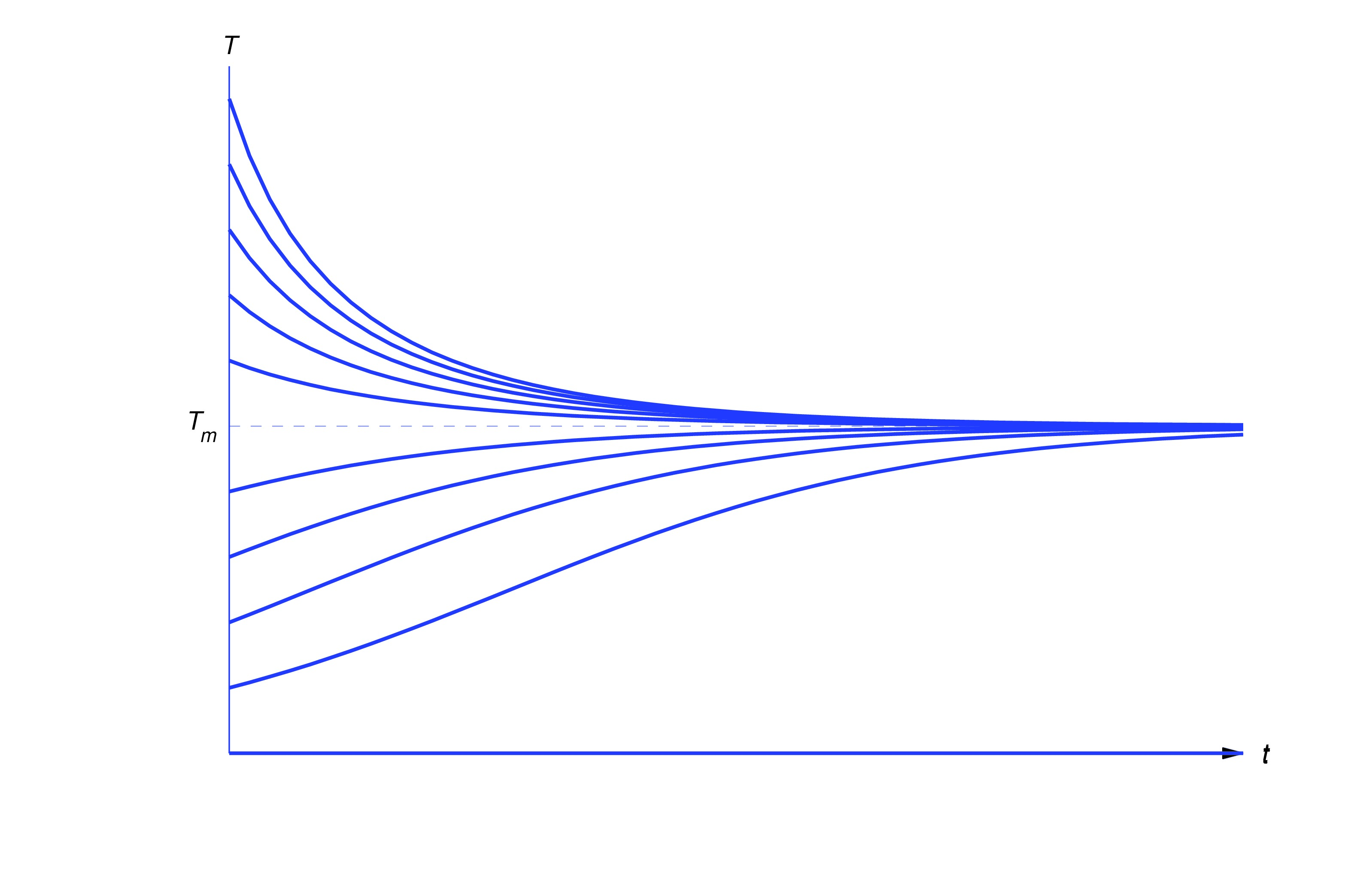
According to Newton’s law of cooling, the temperature of a body changes at a rate proportional to the difference between the temperature of the body and the temperature of the surrounding medium. Thus, if is the temperature of the medium and is the temperature of the body at time , then
where is a positive constant and the minus sign indicates; that the temperature of the body increases with time if it’s less than the temperature of the medium, or decreases if it’s greater. We’ll see in Trench 4.2 that if is constant then the solution of (eq:1.1.5) is where is the temperature of the body when . Therefore , independent of . (Common sense suggests this. Why?)In the long run, the temperature of the body will approach the temperature of the environment, regardless of the initial temperature of the body.
Press the arrow on the right to see the answer.
The figure below shows typical graphs of versus for various values of .
Assuming that the medium remains at constant temperature seems reasonable if we’re considering a cup of coffee cooling in a room, but not if we’re cooling a huge cauldron of molten metal in the same room. The difference between the two situations is that the heat lost by the coffee isn’t likely to raise the temperature of the room appreciably, but the heat lost by the cooling metal is. In this second situation we must use a model that accounts for the heat exchanged between the object and the medium. Let and be the temperatures of the object and the medium respectively, and let and be their initial values. Again, we assume that and are related by (eq:1.1.5). We also assume that the change in heat of the object as its temperature changes from to is and the change in heat of the medium as its temperature changes from to is , where and are positive constants depending upon the masses and thermal properties of the object and medium respectively. If we assume that the total heat of the in the object and the medium remains constant (that is, energy is conserved), then Solving this for and substituting the result into (eq:1.1.6) yields the differential equation for the temperature of the object. After learning to solve linear first order equations, you’ll be able to find that
Glucose Absorption by the Body
Glucose is absorbed by the body at a rate proportional to the amount of glucose present in the bloodstream. Let denote the (positive) constant of proportionality. Suppose there are units of glucose in the bloodstream when , and let be the number of units in the bloodstream at time . Then, since the glucose being absorbed by the body is leaving the bloodstream, satisfies the equation
From calculus you know that if is any constant then satisfies (eq:1.1.7), so (eq:1.1.7) has infinitely many solutions. Setting in (eq:1.1.8) and requiring that yields , soNow let’s complicate matters by injecting glucose intravenously at a constant rate of units of glucose per unit of time. Then the rate of change of the amount of glucose in the bloodstream per unit time is
where the first term on the right is due to the absorption of the glucose by the body and the second term is due to the injection. Later, you’ll be able to solve the equation and find that the solution of (eq:1.1.9) that satisfies is Graphs of this function are similar to those we saw in connection to Newton’s Law of Cooling. (Why?)In each case, the limit as is a constant.
Click on the arrow to the right to see answer.
Use the interactive graph below to explore the behavior of solutions as you change different parameters.
Spread of Epidemics
One model for the spread of epidemics assumes that the number of people infected changes at a rate proportional to the product of the number of people already infected and the number of people who are susceptible, but not yet infected. Therefore, if denotes the total population of susceptible people and denotes the number of infected people at time , then is the number of people who are susceptible, but not yet infected. Thus, where is a positive constant. Assuming that , the solution of this equation is Graphs of this function are similar to those we saw in connection to population growth and decay. (Why?)
Once again, the limit as is a constant.
Click on the arrow to the right to see answer.
Since , this model predicts that all the susceptible people eventually become infected.
Use the interactive graph below to explore the behavior of solutions as you change different parameters.
Newton’s Second Law of Motion
According to Newton’s second law of motion, the instantaneous acceleration of an object with constant mass is related to the force acting on the object by the equation . For simplicity, let’s assume that and the motion of the object is along a vertical line. Let be the displacement of the object from some reference point on Earth’s surface, measured positive upward. In many applications, there are three kinds of forces that may act on the object:
- (a)
- A force such as gravity that depends only on the position , which we write as , where if .
- (b)
- A force such as atmospheric resistance that depends on the position and velocity of the object, which we write as , where is a nonnegative function and we’ve put “outside” to indicate that the resistive force is always in the direction opposite to the velocity.
- (c)
- A force , exerted from an external source (such as a towline from a helicopter) that depends only on .
In this case, Newton’s second law implies that which is usually rewritten as Since the second (and no higher) order derivative of occurs in this equation, we say that it is a second order differential equation.
Interacting Species: Competition
Let and be the populations of two species at time , and assume that each population would grow exponentially if the other didn’t exist; that is, in the absence of competition we would have
where and are positive constants. One way to model the effect of competition is to assume that the growth rate per individual of each population is reduced by an amount proportional to the other population, so (eq:1.1.10) is replaced by
Text Source
Trench, William F., ”Elementary Differential Equations” (2013). Faculty Authored and Edited Books & CDs. 8. (CC-BY-NC-SA)