Introduction to Systems of Differential Equations
Many physical situations are modelled by systems of differential equations in unknown functions, where . The next three examples illustrate physical problems that lead to systems of differential equations. In these examples and throughout this chapter we’ll denote the independent variable by .
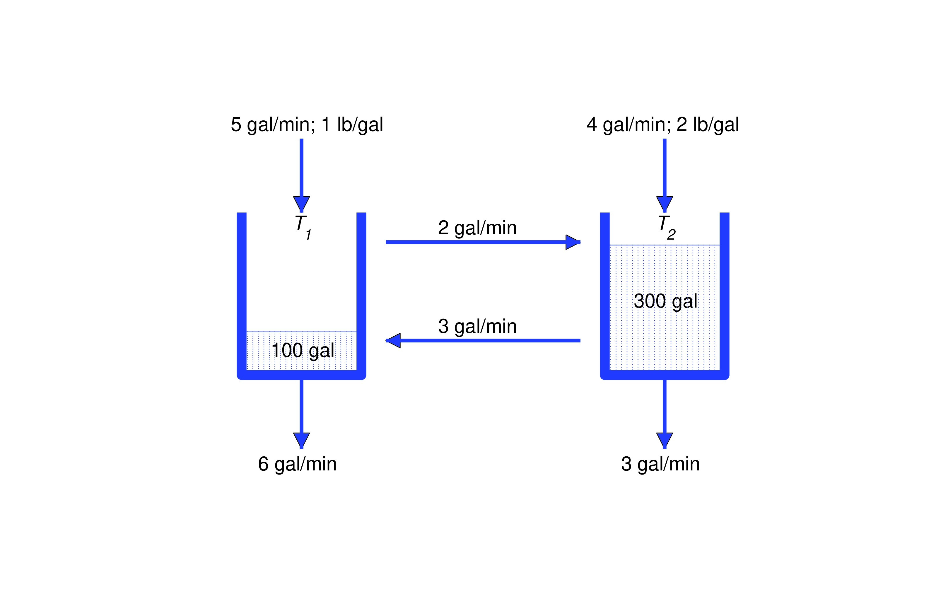
A solution with pound of salt per gallon is pumped into from an external source at gal/min, and a solution with pounds of salt per gallon is pumped into from an external source at gal/min. The solution from is pumped into at 2 gal/min, and the solution from is pumped into at gal/min. is drained at gal/min and is drained at 3 gal/min. Let and be the number of pounds of salt in and , respectively, at time . Derive a system of differential equations for and . Assume that both mixtures are well stirred.
receives salt from the external source at the rate of and from at the rate of Therefore
Solution leaves at the rate of 8 gal/min, since 6 gal/min are drained and 2 gal/min are pumped to ; hence, Eqns. (eq:10.1.1) and (eq:10.1.2) imply thatreceives salt from the external source at the rate of and from at the rate of Therefore
Solution leaves at the rate of gal/min, since gal/min are drained and gal/min are pumped to ; hence, Eqns. (eq:10.1.4) and (eq:10.1.5) imply thatWe say that (eq:10.1.3) and (eq:10.1.6) form a system of two first order equations in two unknowns, and write them together as
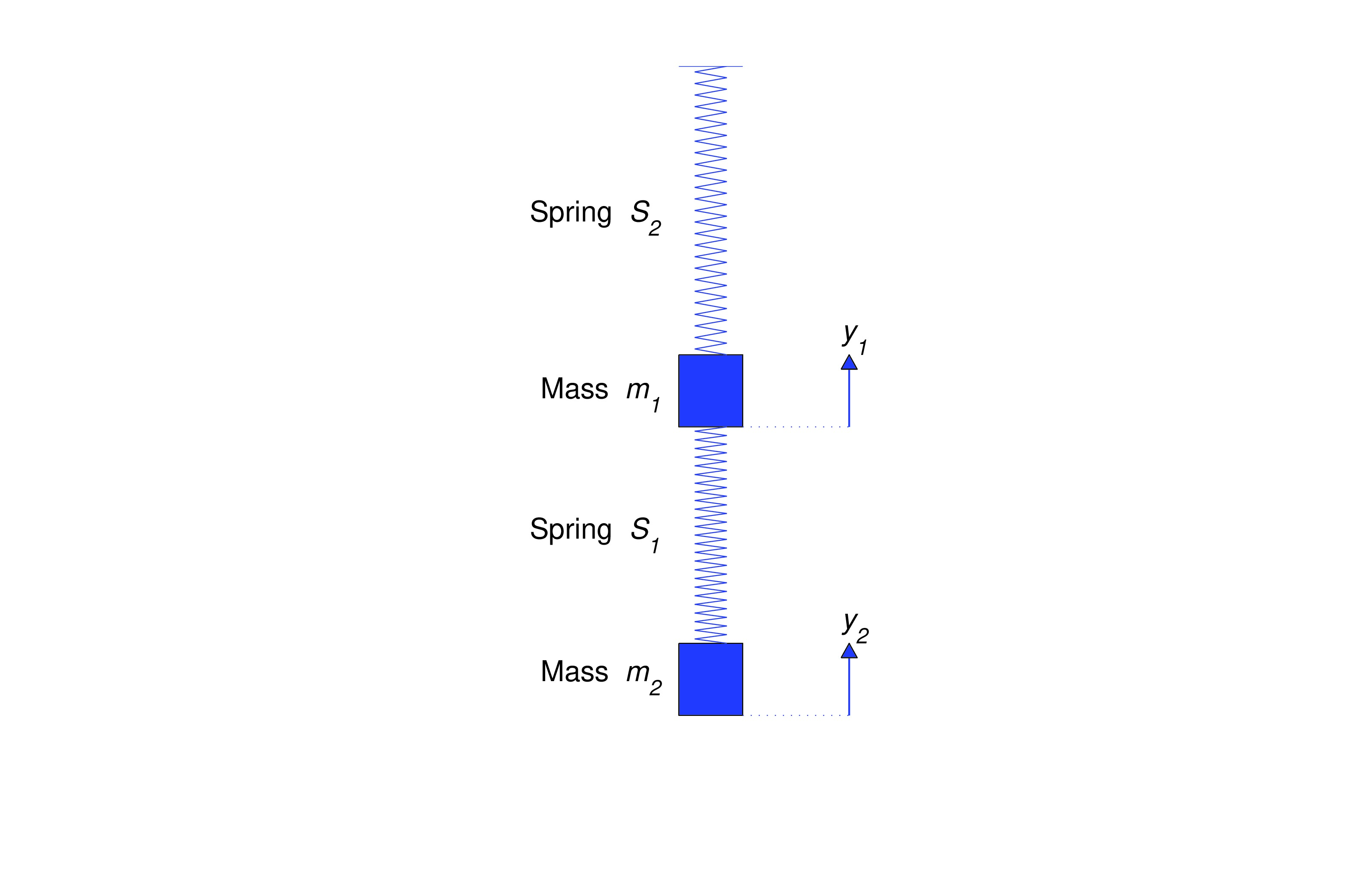
The springs obey Hooke’s law, with spring constants and . Internal friction causes the springs to exert damping forces proportional to the rates of change of their lengths, with damping constants and . Let and be the displacements of the two masses from their equilibrium positions at time , measured positive upward. Derive a system of differential equations for and , assuming that the masses of the springs are negligible and that vertical external forces and also act on the objects.
Let be the Hooke’s law force acting on , and let be the damping force on . Similarly, let and be the Hooke’s law and damping forces acting on . According to Newton’s second law of motion,
When the displacements are and , the change in length of is and the change in length of is . Both springs exert Hooke’s law forces on , while only exerts a Hooke’s law force on . These forces are in directions that tend to restore the springs to their natural lengths. Therefore When the velocities are and , and are changing length at the rates and , respectively. Both springs exert damping forces on , while only exerts a damping force on . Since the force due to damping exerted by a spring is proportional to the rate of change of length of the spring and in a direction that opposes the change, it follows thatFrom (eq:10.1.8), (eq:10.1.9), and (eq:10.1.10),
and From (eq:10.1.7), Therefore we can rewrite (eq:10.1.11) and (eq:10.1.12) as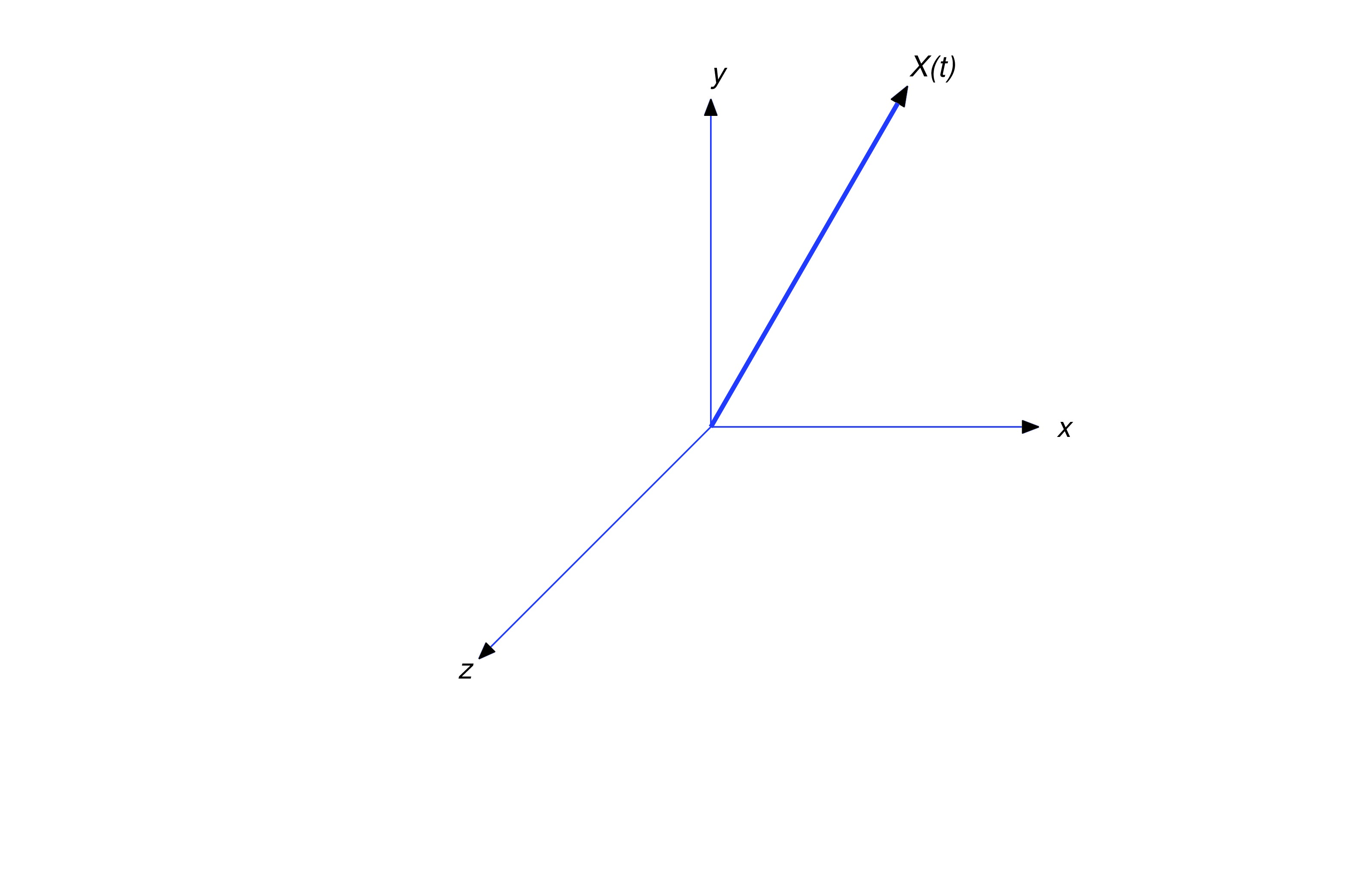
According to Newton’s law of gravitation, Earth’s gravitational force on the object is inversely proportional to the square of the distance of the object from Earth’s center, and directed toward the center; thus,
where is a constant. To determine , we observe that the magnitude of is Let be Earth’s radius. Since when the object is at Earth’s surface, Therefore we can rewrite (eq:10.1.13) as Now suppose is the only force acting on the object. According to Newton’s second law of motion, ; that is, Cancelling the common factor and equating components on the two sides of this equation yields the systemRewriting Higher Order Systems as First Order Systems
A system of the form
is called a first order system, since the only derivatives occurring in it are first derivatives. The derivative of each of the unknowns may depend upon the independent variable and all the unknowns, but not on the derivatives of other unknowns. When we wish to emphasize the number of unknown functions in (eq:10.1.15) we will say that (eq:10.1.15) is an system.Systems involving higher order derivatives can often be reformulated as first order systems by introducing additional unknowns. The next two examples illustrate this.
Rewriting Scalar Differential Equations as Systems
In this chapter we’ll refer to differential equations involving only one unknown function as scalar differential equations. Scalar differential equations can be rewritten as systems of first order equations by the method illustrated in the next two examples.
Since systems of differential equations involving higher derivatives can be rewritten as first order systems by the method used in Examples example:10.1.5 –example:10.1.7 , we’ll consider only first order systems.
Numerical Solution of Systems
The numerical methods that we studied in Chapter 3 can be extended to systems, and most differential equation software packages include programs to solve systems of equations. We won’t go into detail on numerical methods for systems; however, for illustrative purposes we’ll describe the Runge-Kutta method for the numerical solution of the initial value problem
Text Source
Trench, William F., ”Elementary Differential Equations” (2013). Faculty Authored and Edited Books & CDs. 8. (CC-BY-NC-SA)