We study the motion of a object moving under the influence of a central force.
Motion Under A Central Force
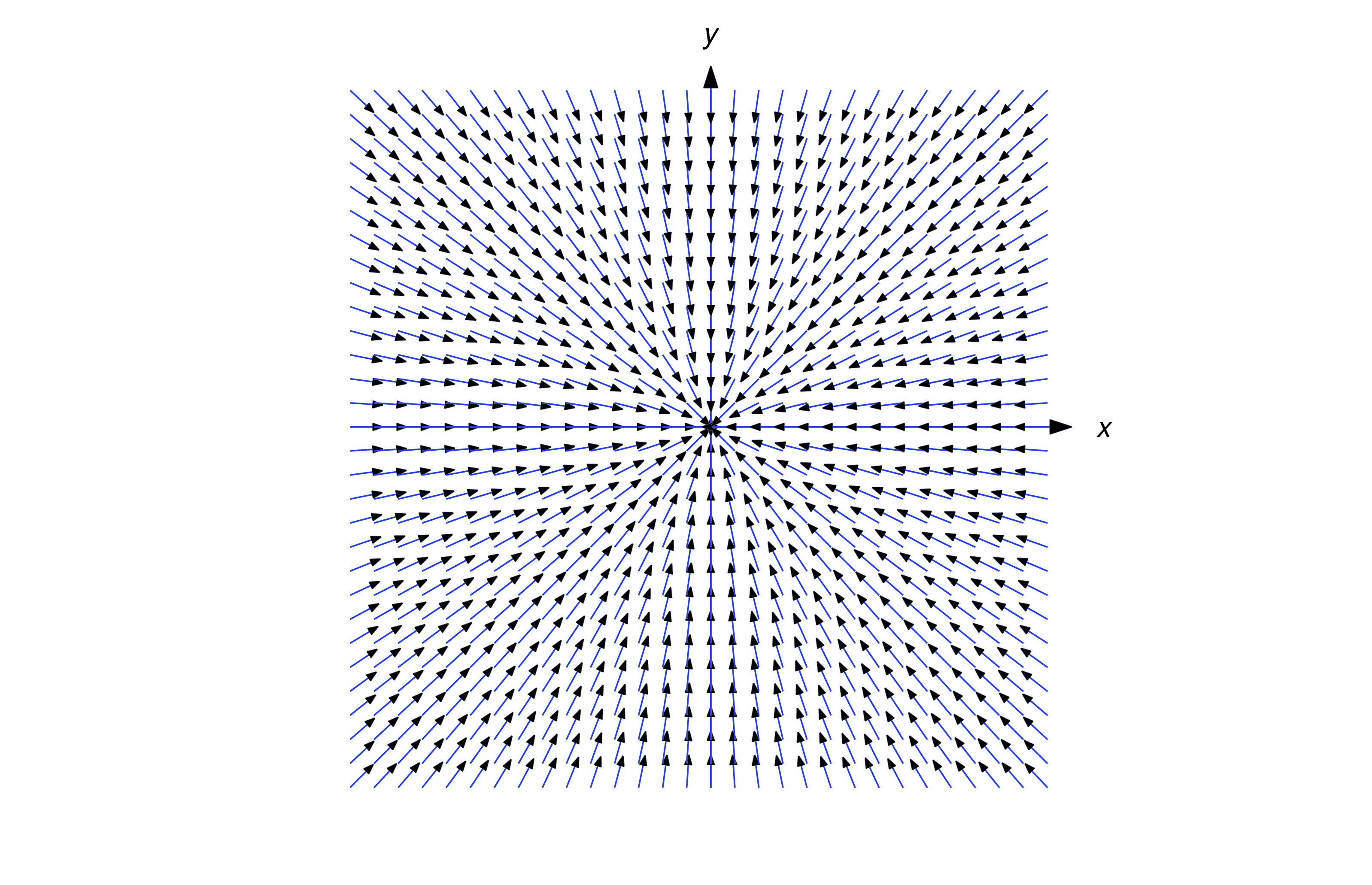
We’ll now study the motion of a object moving under the influence of a central force; that is, a force whose magnitude at any point other than the origin depends only on the distance from to the origin, and whose direction at is parallel to the line connecting and the origin, as indicated in the figure below for the case where the direction of the force at every point is toward the origin.
Gravitational forces are central forces; for example, as mentioned in Trench 4.3, if we assume that Earth is a perfect sphere with constant mass density then Newton’s law of gravitation asserts that the force exerted on an object by Earth’s gravitational field is proportional to the mass of the object and inversely proportional to the square of its distance from the center of Earth, which we take to be the origin.
If the initial position and velocity vectors of an object moving under a central force are parallel, then the subsequent motion is along the line from the origin to the initial position. Here we’ll assume that the initial position and velocity vectors are not parallel; in this case the subsequent motion is in the plane determined by them. For convenience we take this to be the -plane. We’ll consider the problem of determining the curve traversed by the object. We call this curve the orbit.
We can represent a central force in terms of polar coordinates as We assume that is continuous for all . The magnitude of at is , so it depends only on the distance from the point to the origin the direction of is from the point to the origin if , or from the origin to the point if . We’ll show that the orbit of an object with mass moving under this force is given by where is solution of the differential equation
and is a constant defined below.Newton’s second law of motion () says that the polar coordinates and of the particle satisfy the vector differential equation
To deal with this equation we introduce the unit vectors Note that points in the direction of increasing and points in the direction of increasing . (See the figure below)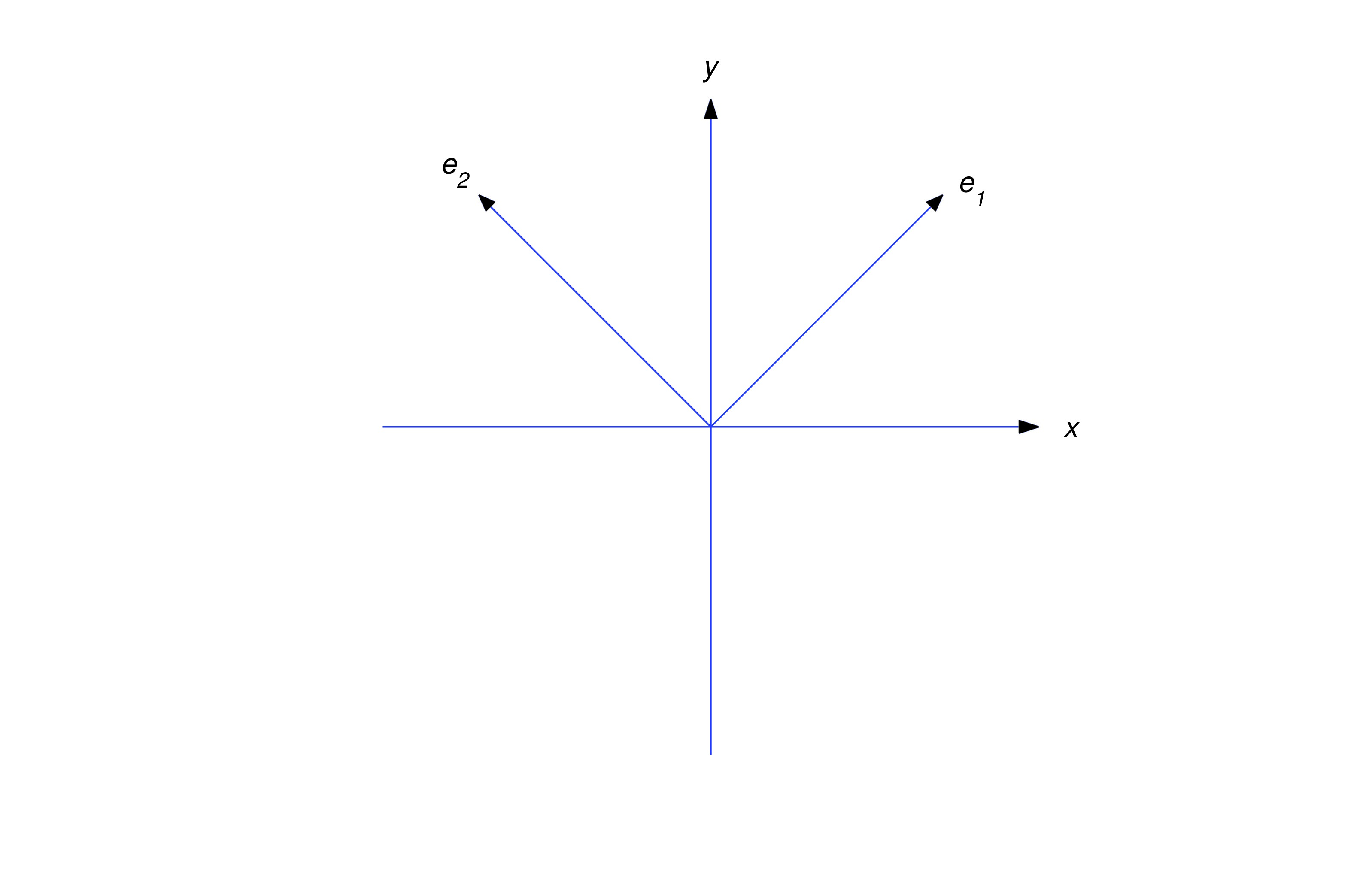
Moreover,
and so and are perpendicular. Recalling that the single prime stands for differentiation with respect to , we see from (eq:6.4.3) and the chain rule thatNow we can write (eq:6.4.2) as
But (from (eq:6.4.4)), andNow let . Then (from (eq:6.4.7)) and which implies that
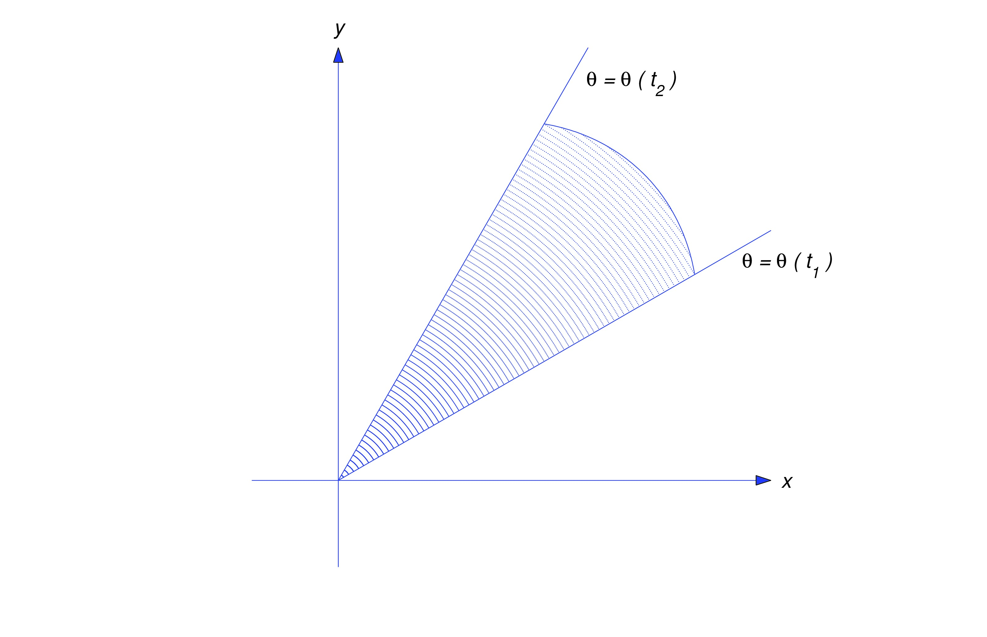
since Differentiating (eq:6.4.8) with respect to yields which implies that Substituting from these equalities into (eq:6.4.6) and recalling that yields and dividing through by yields (eq:6.4.1).Eqn. (eq:6.4.7) has the following geometrical interpretation, which is known as Kepler’s Second Law.
Motion Under an Inverse Square Law Force
In the special case where , so can be interpreted as a gravitational force, (eq:6.4.1) becomes
The general solution of the complementary equation can be written in amplitude–phase form as where and is a phase angle. Since is a particular solution of (eq:6.4.10), the general solution of (eq:6.4.10) is hence, the orbit is given by which we rewrite as where A curve satisfying (eq:6.4.11) is a conic section with a focus at the origin. The nonnegative constant is the eccentricity of the orbit, which is an ellipse if ellipse (a circle if ), a parabola if , or a hyperbola if .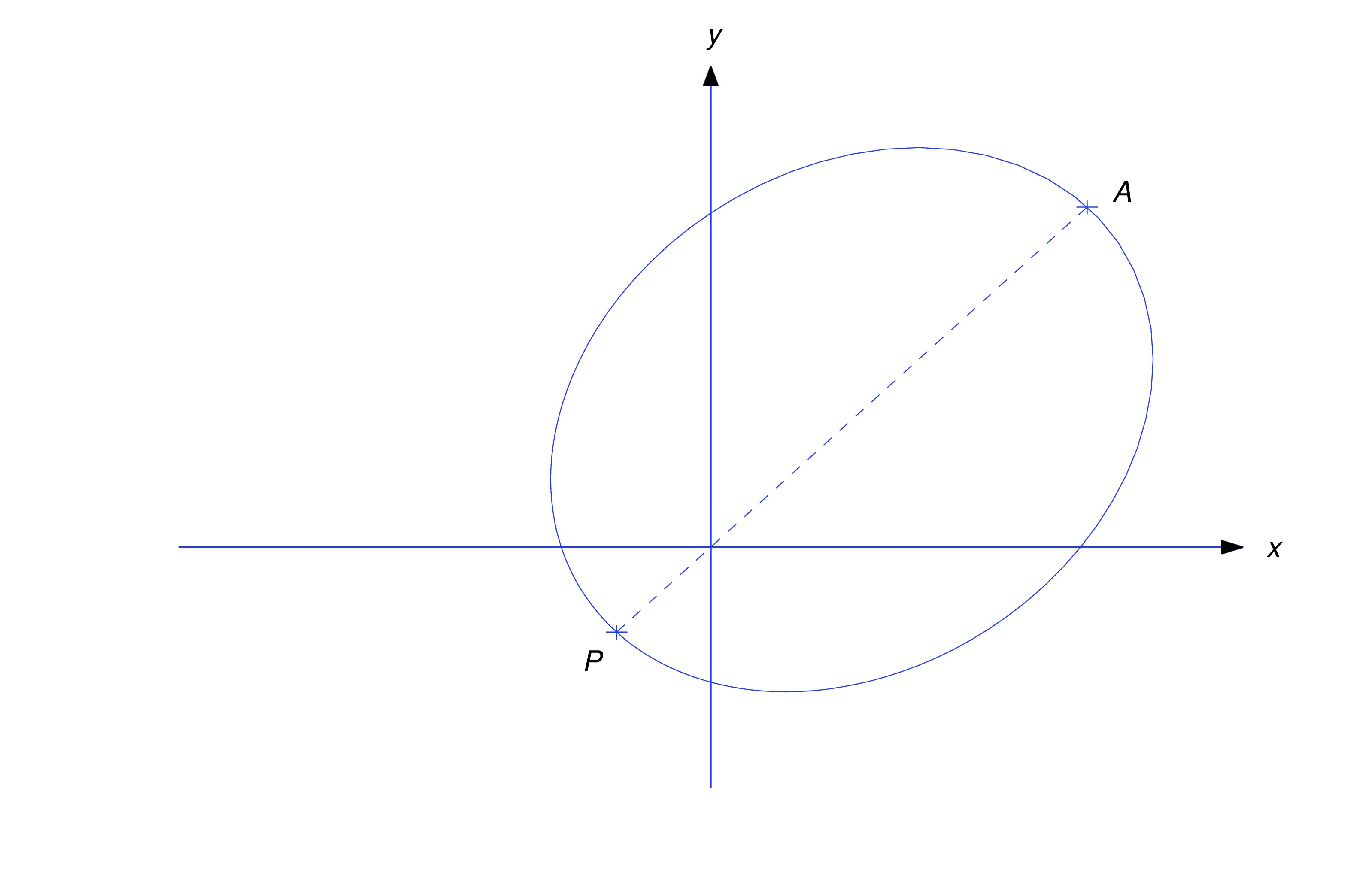
If the orbit is an ellipse, then the minimum and maximum values of are
shows a typical elliptic orbit. The point on the orbit where is the perigee and the point where is the apogee.
For example, Earth’s orbit around the Sun is approximately an ellipse with , miles, and miles. Halley’s comet has a very elongated approximately elliptical orbit around the sun, with , miles, and miles. Some comets (the nonrecurring type) have parabolic or hyperbolic orbits.
Text Source
Trench, William F., ”Elementary Differential Equations” (2013). Faculty Authored and Edited Books & CDs. 8. (CC-BY-NC-SA)