We learn how to recognize whether or not a first-order equation is exact. We also learn how to solve an exact equation.
Exact Equations
In this section it’s convenient to write first order differential equations in the form
This equation can be interpreted as where is the independent variable and is the dependent variable, or as where is the independent variable and is the dependent variable. Since the solutions of (eq:2.5.2) and (eq:2.5.3) will often have to be left in implicit form, we’ll say that is an implicit solution of (eq:2.5.1) if every differentiable function that satisfies is a solution of (eq:2.5.2) and every differentiable function that satisfies is a solution of (eq:2.5.3).Here are some examples:
Note that a separable equation can be written as (eq:2.5.1) as
We’ll develop a method for solving (eq:2.5.1) under appropriate assumptions on and . This method is an extension of the method of separation of variables. Before stating it we consider an example.
You may think this example is pointless, since concocting a differential equation that has a given implicit solution isn’t particularly interesting. However, it illustrates the next important theorem, which we’ll prove by using implicit differentiation, as in Example example:2.5.1.
- Proof
- Regarding as a function of and differentiating (eq:2.5.6) implicitly with respect to yields On the other hand, regarding as a function of and differentiating (eq:2.5.6) implicitly with respect to yields Thus, (eq:2.5.6) is an implicit solution of (eq:2.5.7) in either of its two possible interpretations.
We’ll say that the equation
is exact on an an open rectangle if there’s a function such that and are continuous, and for all in . This usage of “exact” is related to its usage in calculus, where the expression (obtained by substituting (eq:2.5.9) into the left side of (eq:2.5.8)) is the exact differential of .Example example:2.5.1 shows that it’s easy to solve (eq:2.5.8) if it’s exact and we know a function that satisfies (eq:2.5.9). The important questions are:
Question 1:
Given an equation (eq:2.5.8), how can we determine whether it’s exact?
Question 2:
If (eq:2.5.8) is exact, how do we find a function satisfying (eq:2.5.9)?
To discover the answer to Question 1, assume that there’s a function that satisfies (eq:2.5.9) on some open rectangle , and in addition that has continuous mixed partial derivatives and . Then a theorem from calculus implies that
If and , differentiating the first of these equations with respect to and the second with respect to yields From (eq:2.5.10) and (eq:2.5.11), we conclude that a necessary condition for exactness is that . This motivates the next theorem, which we state without proof.To help you remember the exactness condition, observe that the coefficients of and are differentiated in (eq:2.5.12) with respect to the “opposite” variables; that is, the coefficient of is differentiated with respect to , while the coefficient of is differentiated with respect to .
The next example illustrates two possible methods for finding a function that satisfies the condition and if is exact.
Method 2: Instead of first integrating (eq:2.5.14) with respect to , we could begin by integrating (eq:2.5.15) with respect to to obtain
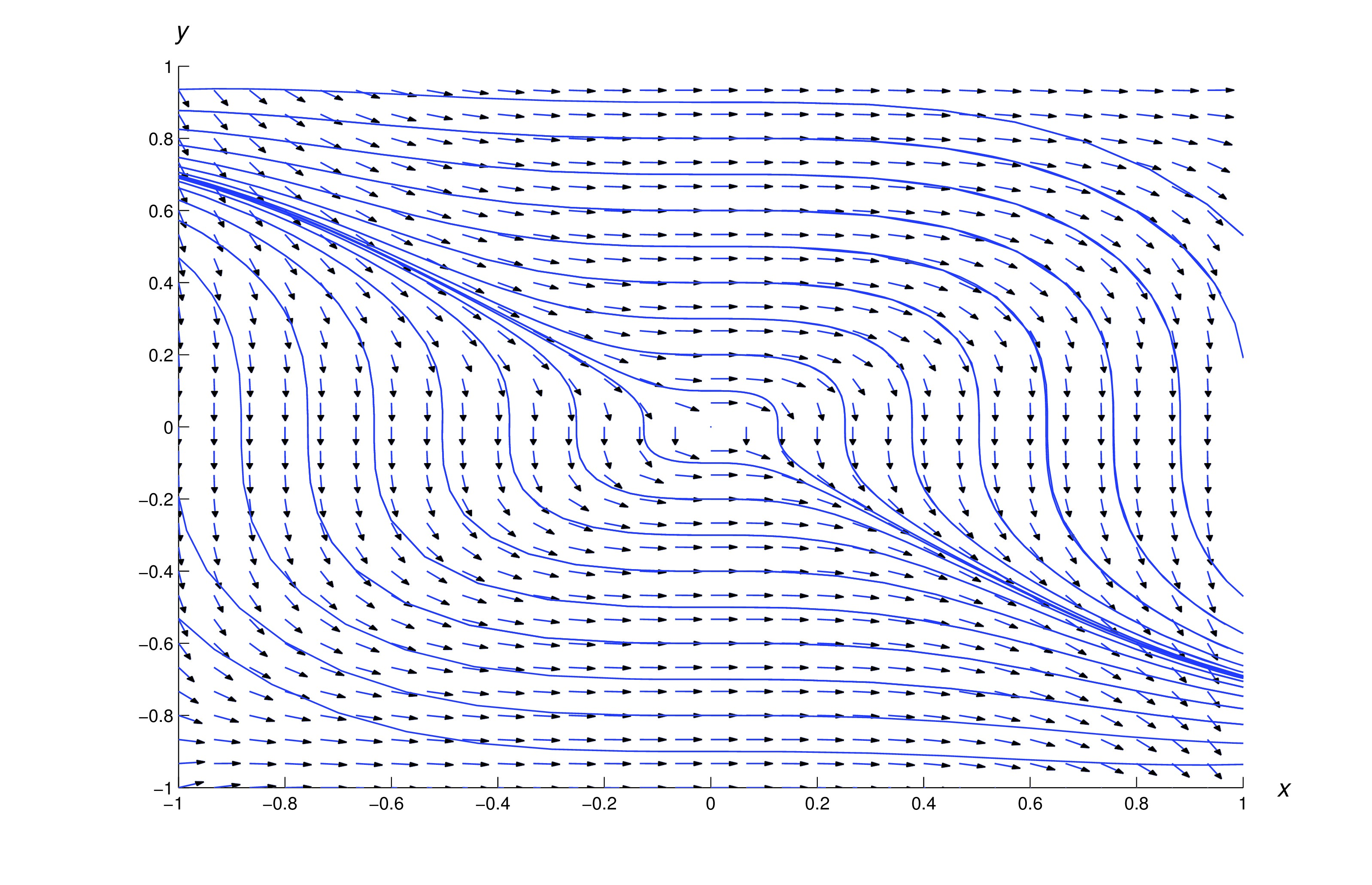
where is an arbitrary function of . To determine , we assume that is differentiable and differentiate with respect to , which yields Comparing this with (eq:2.5.14) shows that Integrating this and again taking the constant of integration to be zero yields Substituting this into (eq:2.5.18) yields (eq:2.5.17).Figure figure:2.5.1 shows a direction field and some integral curves of (eq:2.5.13),
Here’s a summary of the procedure used in Method 1 of this example. You should summarize procedure used in Method 2.
Procedure For Solving An Exact Equation
Step 1. Check that the equation
satisfies the exactness condition . If not, don’t go further with this procedure.Step 2. Integrate with respect to to obtain
where is an antiderivative of with respect to , and is an unknown function of .Step 3. Differentiate (eq:2.5.20) with respect to to obtain
Step 4. Equate the right side of this equation to and solve for ; thus,
Step 5. Integrate with respect to , taking the constant of integration to be zero, and substitute the result in (eq:2.5.20) to obtain .
Step 6. Set to obtain an implicit solution of (eq:2.5.19). If possible, solve for explicitly as a function of .
It’s a common mistake to omit Step 6. However, it’s important to include this step, since isn’t itself a solution of (eq:2.5.19).
Many equations can be conveniently solved by either of the two methods used in Example example:2.5.3. However, sometimes the integration required in one approach is more difficult than in the other. In such cases we choose the approach that requires the easier integration.
Attempting to apply our procedure to an equation that isn’t exact will lead to failure in Step 4, since the function won’t be independent of if , and therefore can’t be the derivative of a function of alone. Here’s an example that illustrates this.
Text Source
Trench, William F., ”Elementary Differential Equations” (2013). Faculty Authored and Edited Books & CDs. 8. (CC-BY-NC-SA)