Constant Coefficient Homogeneous Systems III
We now consider the system , where has a complex eigenvalue with . We continue to assume that has real entries, so the characteristic polynomial of has real coefficients. This implies that is also an eigenvalue of .
An eigenvector of associated with will have complex entries, so we’ll write where and have real entries; that is, and are the real and imaginary parts of . Since ,
Taking complex conjugates here and recalling that has real entries yields which shows that is an eigenvector associated with . The complex conjugate eigenvalues and can be separately associated with linearly independent solutions ; however, we won’t pursue this approach, since solutions obtained in this way turn out to be complex–valued. Instead, we’ll obtain solutions of in the form where and are real–valued scalar functions. The next theorem shows how to do this.
We leave it to you to show from this that and are both nonzero. Substituting from these equations into (eq:10.6.4) yields
The augmented matrix of is which is row equivalent to Therefore and . Taking yields the eigenvector The real and imaginary parts of are which are solutions of (eq:10.6.8). Since the Wronskian of at is is a fundamental set of solutions of (eq:10.6.8). The general solution of (eq:10.6.8) is
The augmented matrix of is which is row equivalent to Therefore and . Taking yields the eigenvector The real and imaginary parts of are which are solutions of (eq:10.6.9). Since the Wronskian of at is is a fundamental set of solutions of (eq:10.6.9). The general solution of (eq:10.6.9) is
Geometric Properties of Solutions when
We’ll now consider the geometric properties of solutions of a constant coefficient system
under the assumptions of this section; that is, when the matrix has a complex eigenvalue () and is an associated eigenvector, where and have real components. To describe the trajectories accurately it’s necessary to introduce a new rectangular coordinate system in the - plane. This raises a point that hasn’t come up before: It is always possible to choose so that . A special effort is required to do this, since not every eigenvector has this property. However, if we know an eigenvector that doesn’t, we can multiply it by a suitable complex constant to obtain one that does. To see this, note that if is a -eigenvector of and is an arbitrary real number, then is also a -eigenvector of , since The real and imaginary parts of are so Therefore if If we can use the quadratic formula to find two real values of such that .Henceforth, we’ll assume that . Let and be unit vectors in the directions of and , respectively; that is, and . The new rectangular coordinate system will have the same origin as the - system. The coordinates of a point in this system will be denoted by , where and are the displacements in the directions of and , respectively.
From (eq:10.6.5), the solutions of (eq:10.6.10) are given by
For convenience, let’s call the curve traversed by a shadow trajectory (eq:10.6.10). Multiplying (eq:10.6.13) by yields where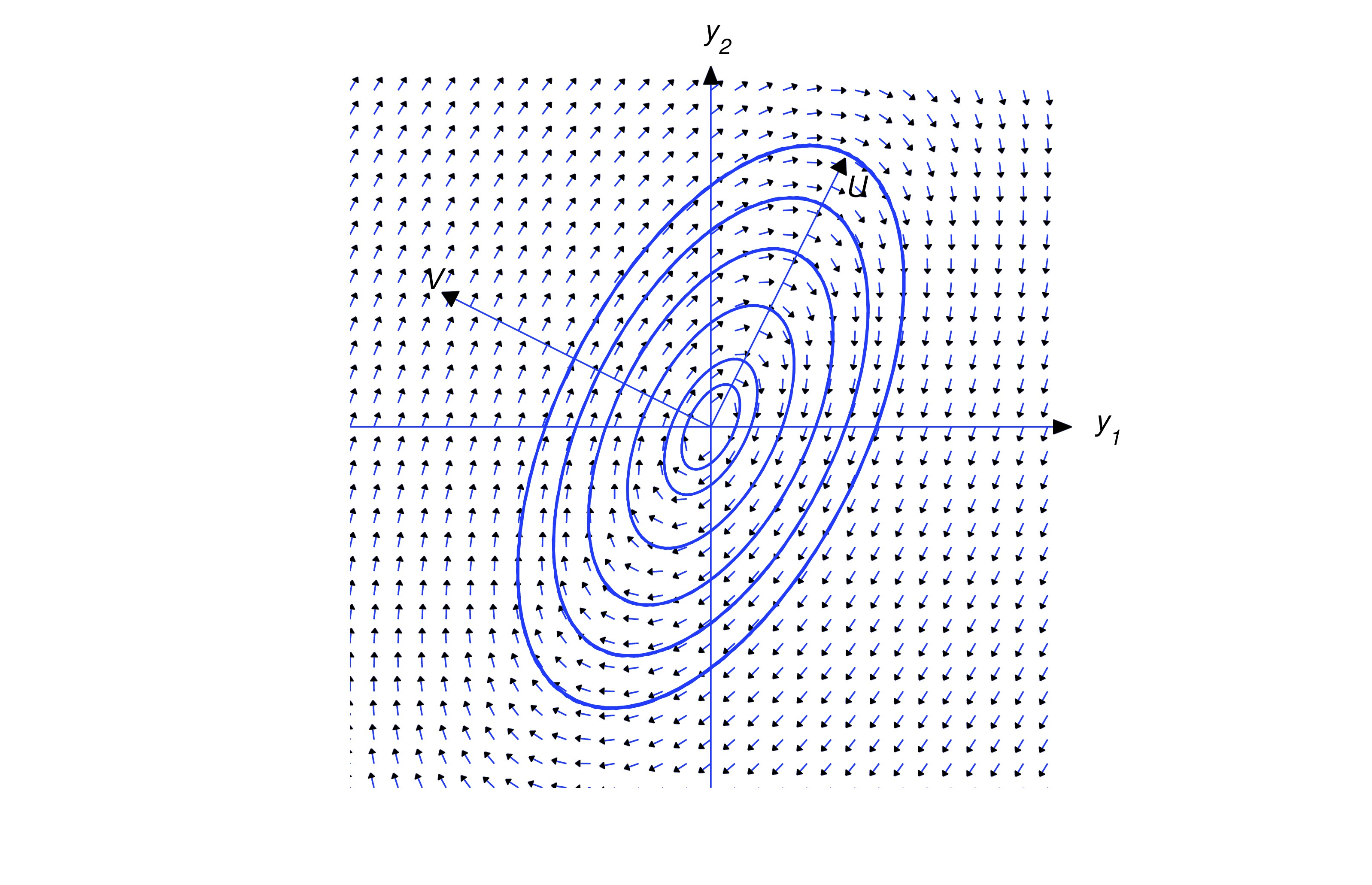
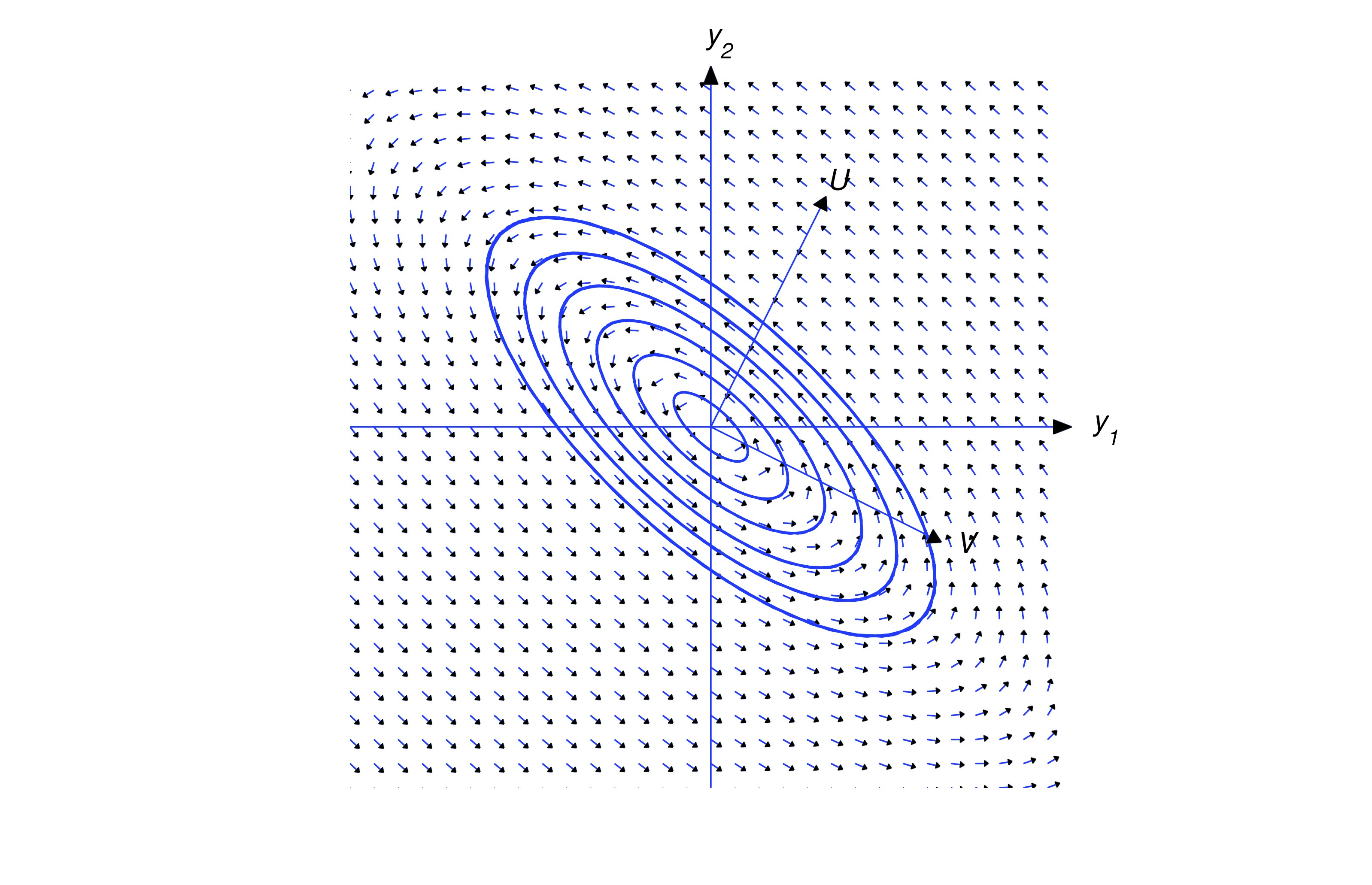
If , then any trajectory of (eq:10.6.10) is a shadow trajectory of (eq:10.6.10); therefore, if is purely imaginary, then the trajectories of (eq:10.6.10) are ellipses traversed periodically as indicated in Figures figure:10.6.1 and figure:10.6.2.
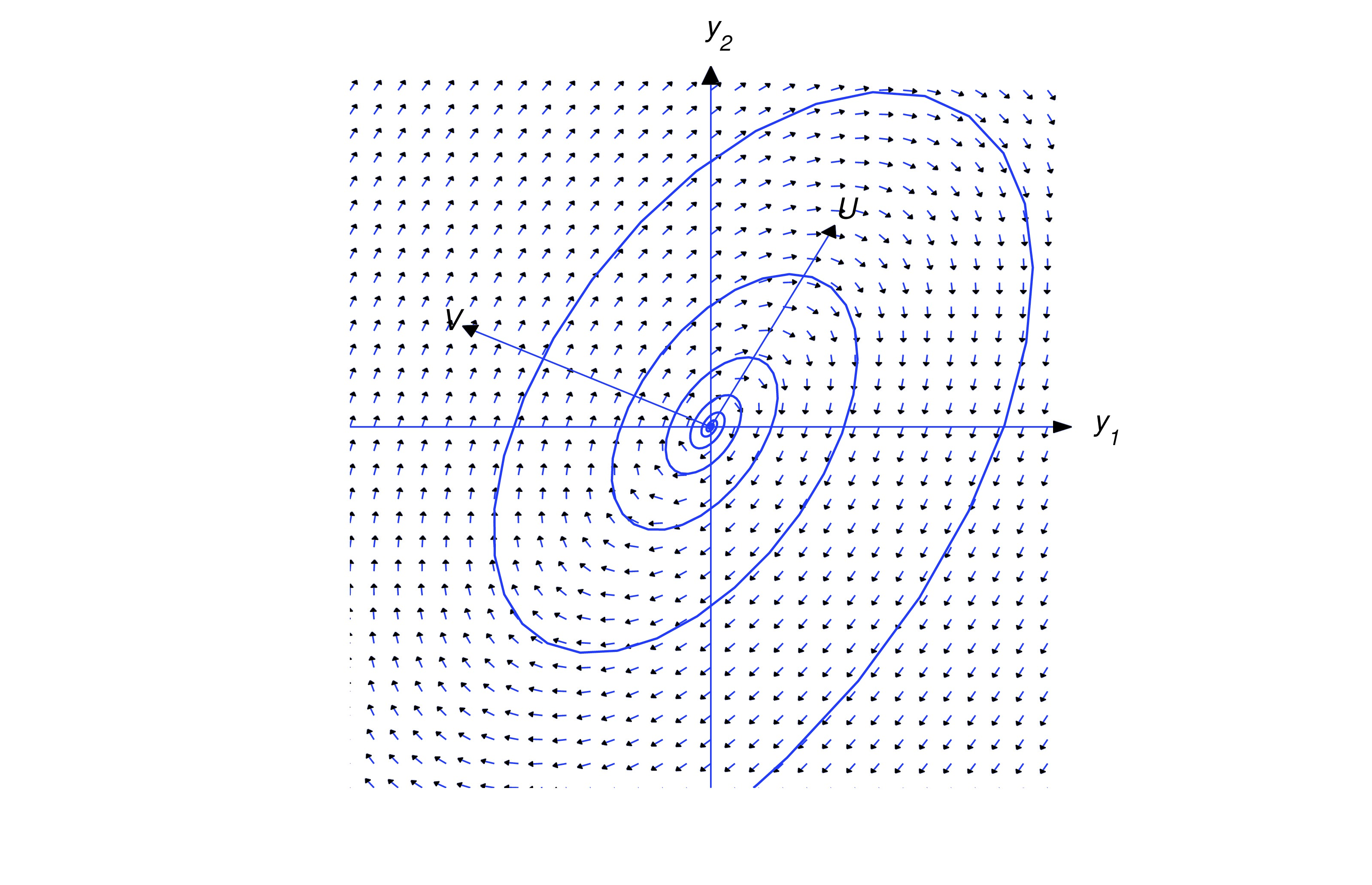
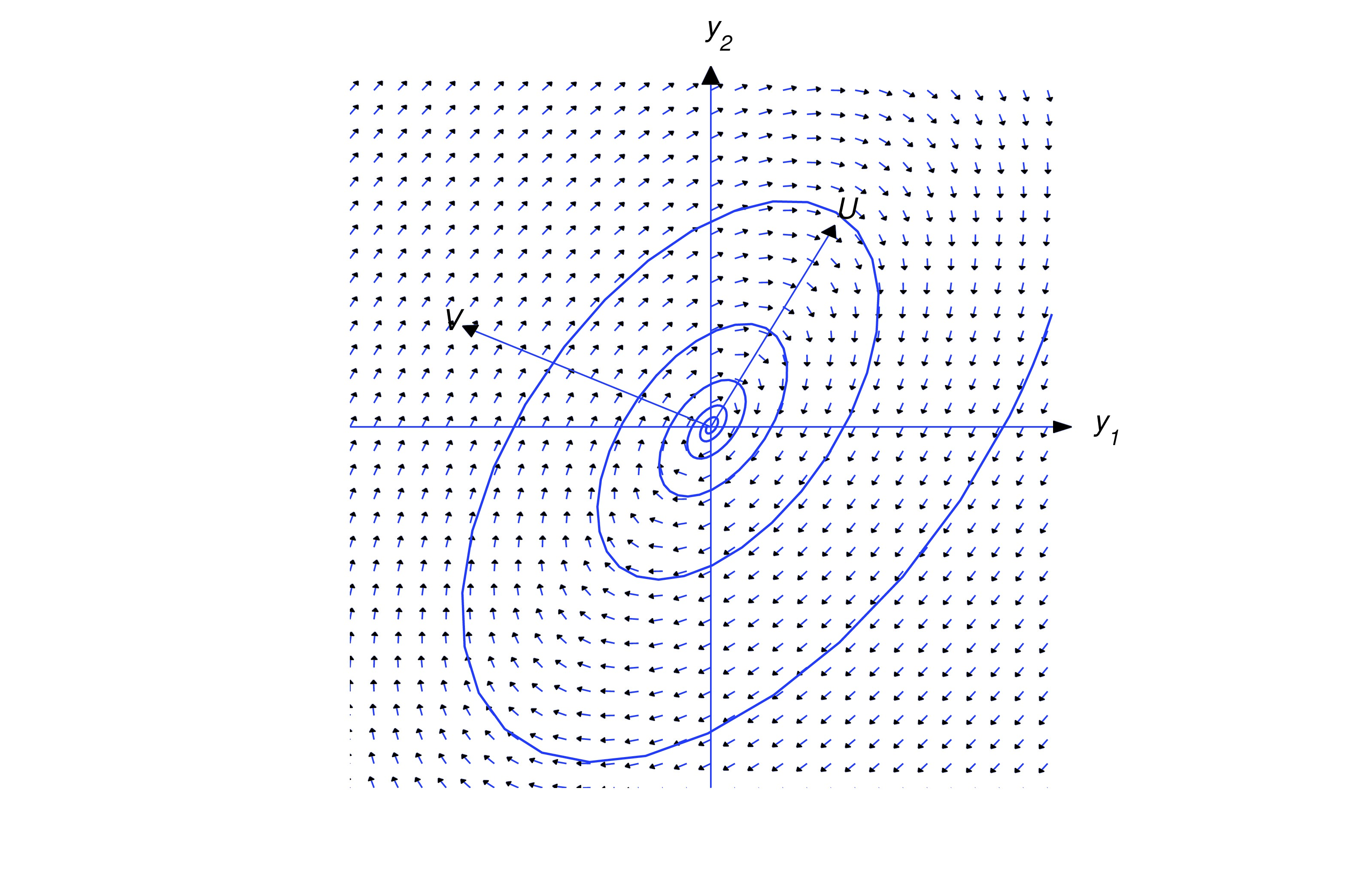
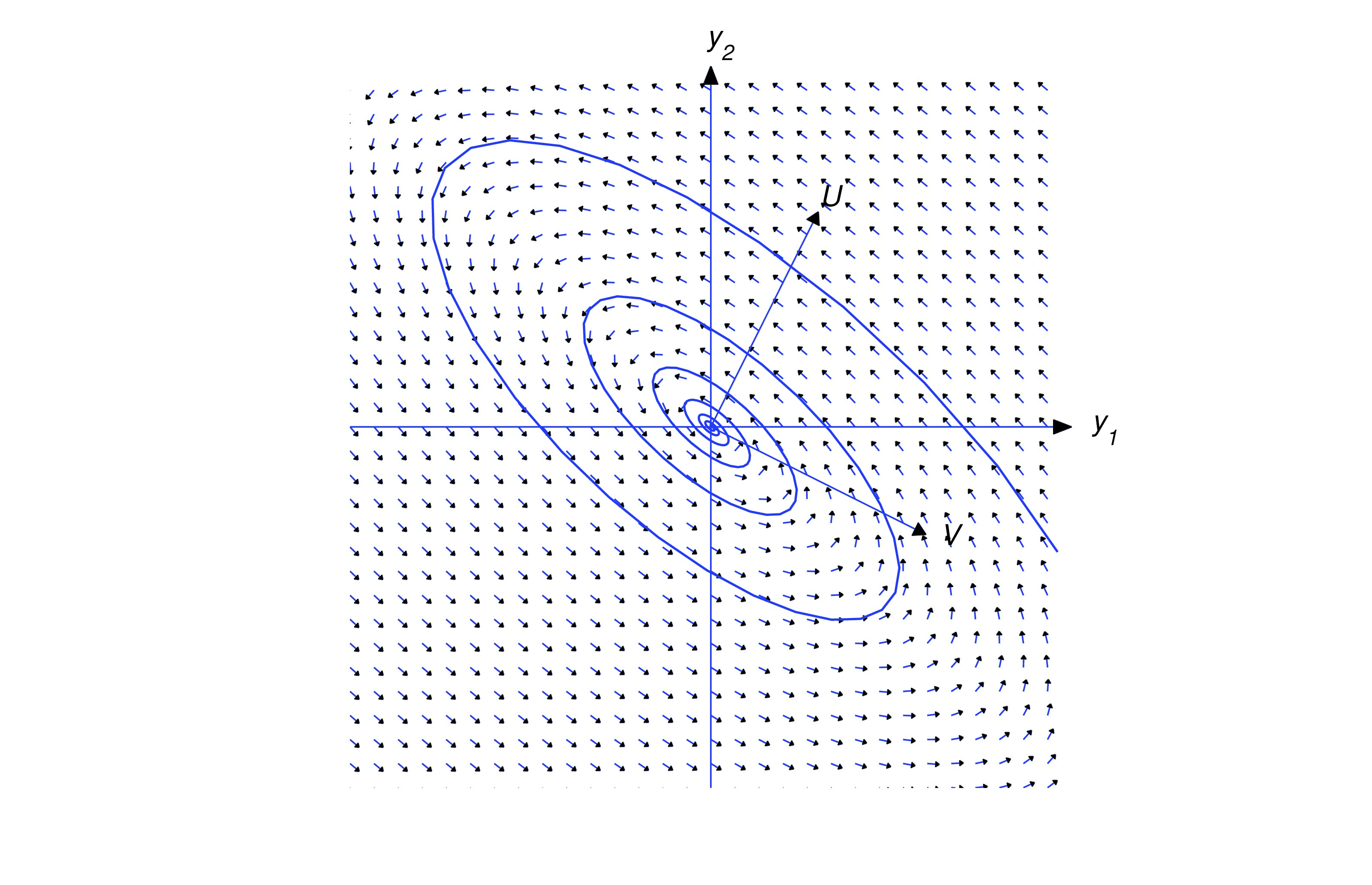
If , then so the trajectory spirals away from the origin as varies from to . The direction of the spiral depends upon the relative orientation of and , as shown in the figures below.
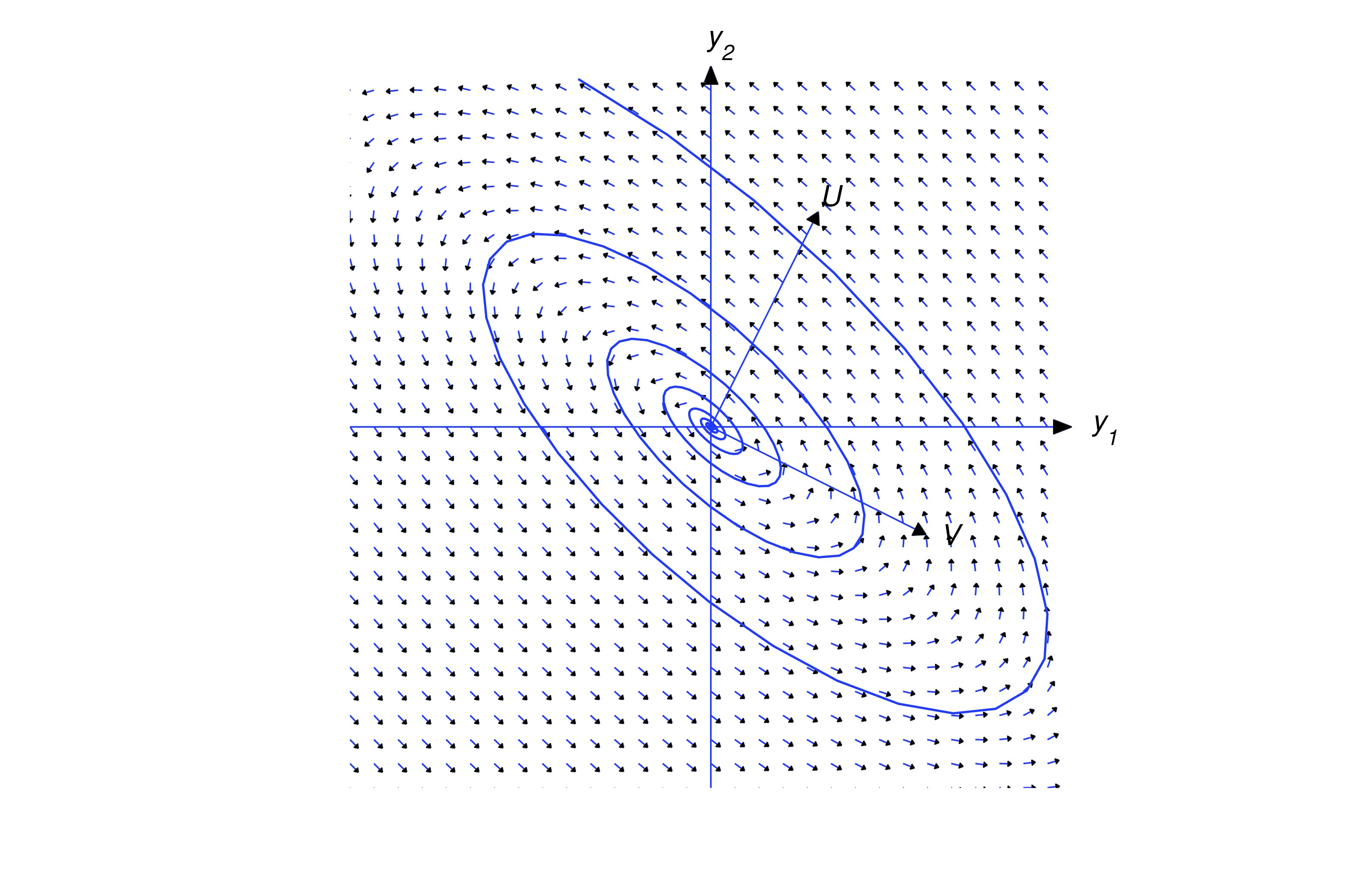
If , then
so the trajectory spirals toward the origin as varies from to . Again, the direction of the spiral depends upon the relative orientation of and , as shown in the figures below.
Text Source
Trench, William F., ”Elementary Differential Equations” (2013). Faculty Authored and Edited Books & CDs. 8. (CC-BY-NC-SA)