We show how multiplying an equation by an integrating factor can make the equation exact, and we give examples where this is a nice technique for solving a first-order equation.
Integrating Factors
In Trench 2.5, Exact Equations, we saw that if , , and are continuous and on an open rectangle then
is exact on . Sometimes an equation that isn’t exact can be made exact by multiplying it by an appropriate function. For example, is not exact, since in (eq:2.6.2). However, multiplying (eq:2.6.2) by yields which is exact, since in (eq:2.6.3). Solving (eq:2.6.3) by Procedure proc:solvingExactEq of Trench 2.5, yields the implicit solutionA function is an integrating factor for (eq:2.6.1) if
is exact. If we know an integrating factor for (eq:2.6.1), we can solve the exact equation (eq:2.6.4) by Procedure proc:solvingExactEq Trench 2.5. It would be nice if we could say that (eq:2.6.1) and (eq:2.6.4) always have the same solutions, but this isn’t so. For example, a solution of (eq:2.6.4) such that on some interval could fail to be a solution of (eq:2.6.1) , while (eq:2.6.1) may have a solution such that isn’t even defined . Similar comments apply if is the independent variable and is the dependent variable in (eq:2.6.1) and (eq:2.6.4). However, if is defined and nonzero for all , (eq:2.6.1) and (eq:2.6.4) are equivalent; that is, they have the same solutions.Finding Integrating Factors
By applying Theorem thmtype:2.5.2 (with and replaced by and ), we see that (eq:2.6.4) is exact on an open rectangle if , , , and are continuous and on . It’s better to rewrite the last equation as
which reduces to the known result for exact equations; that is, if then (eq:2.6.5) holds with , so (eq:2.6.1) is exact.You may think (eq:2.6.5) is of little value, since it involves partial derivatives of the unknown integrating factor , and we haven’t studied methods for solving such equations. However, we’ll now show that (eq:2.6.5) is useful if we restrict our search to integrating factors that are products of a function of and a function of ; that is, . We’re not saying that every equation has an integrating factor of this form; rather, we’re saying that some equations have such integrating factors. We’ll now develop a way to determine whether a given equation has such an integrating factor, and a method for finding the integrating factor in this case.
If , then and , so (eq:2.6.5) becomes
or, after dividing through by , Now let so (eq:2.6.7) becomesWe obtained (eq:2.6.8) by assuming that has an integrating factor . However, we can now view (eq:2.6.7) differently: If there are functions and that satisfy (eq:2.6.8) and we define
then reversing the steps that led from (eq:2.6.6) to (eq:2.6.8) shows that is an integrating factor for . In using this result, we take the constants of integration in (eq:2.6.9) to be zero and choose the signs conveniently so the integrating factor has the simplest form.There’s no simple general method for ascertaining whether functions and satisfying (eq:2.6.8) exist. However, the next theorem gives simple sufficient conditions for the given equation to have an integrating factor that depends on only one of the independent variables and , and for finding an integrating factor in this case.
- (a)
- If is independent of on and we define then is an integrating factor for on
- (b)
- If is independent of on and we define then is an integrating factor for (eq:2.6.11) on
- Proof
- item:2.6.1a If is independent of , then (eq:2.6.8) holds with and . Therefore
so (eq:2.6.10) is an integrating factor for (eq:2.6.11) on .
item:2.6.1b If is independent of then eqrefeq:2.6.8 holds with and , and a similar argument shows that (eq:2.6.12) is an integrating factor for (eq:2.6.11) on .
The next two examples show how to apply Theorem thmtype:2.6.1.
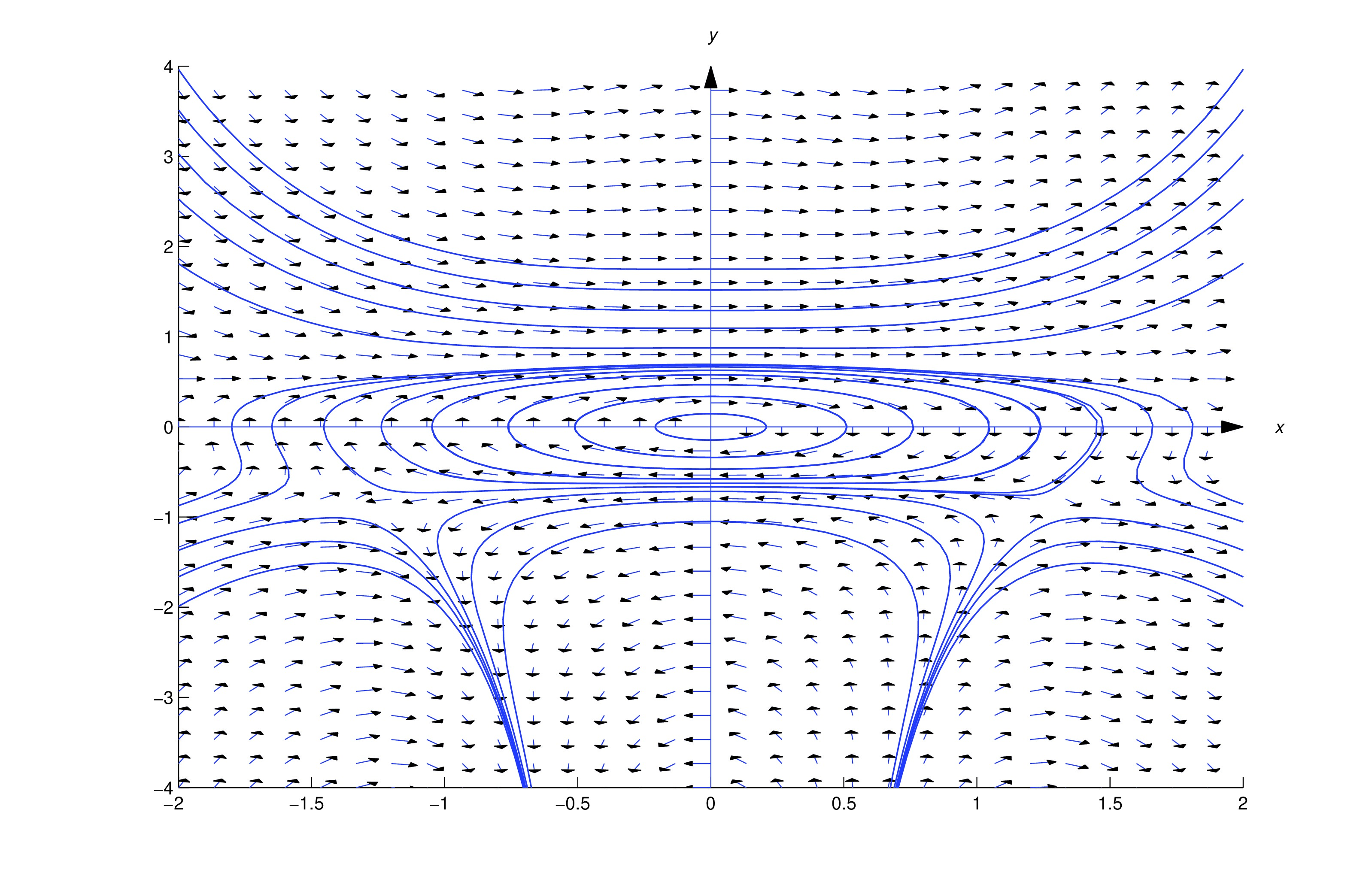
To solve this equation, we must find a function such that
and Integrating (eq:2.6.16) with respect to yields Differentiating this with respect to yields Comparing this with (eq:2.6.15) shows that ; therefore, we can let in (eq:2.6.17) and conclude that is an implicit solution of (eq:2.6.14). It is also an implicit solution of (eq:2.6.13).The figure below shows a direction field and some integral curves for (eq:2.6.13)
Theorem thmtype:2.6.1 does not apply in the next example, but the more general argument that led to Theorem thmtype:2.6.1 provides an integrating factor.
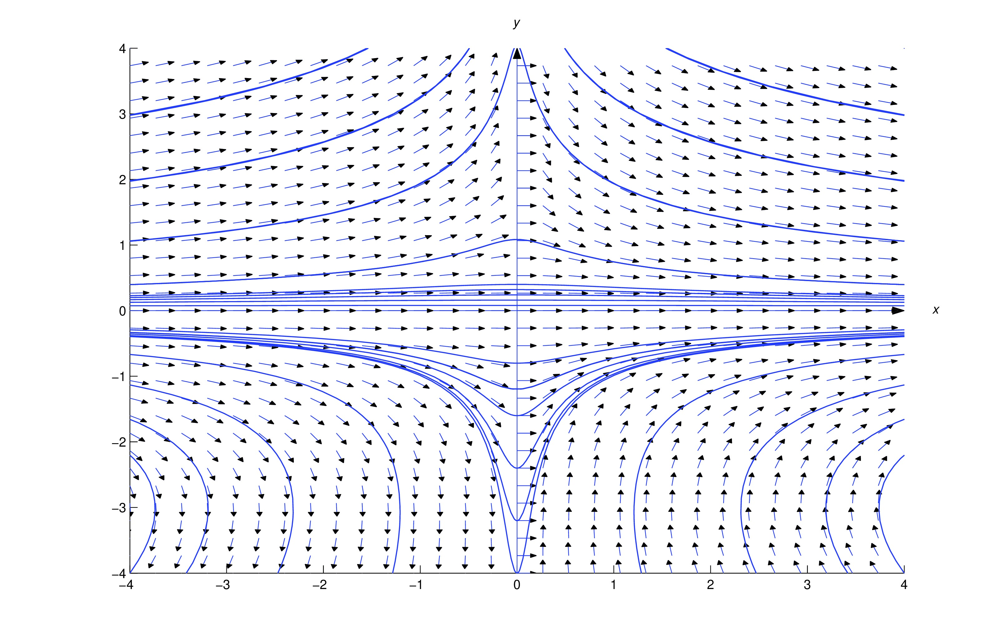
The figure below shows a direction field and integral curves for (eq:2.6.23).
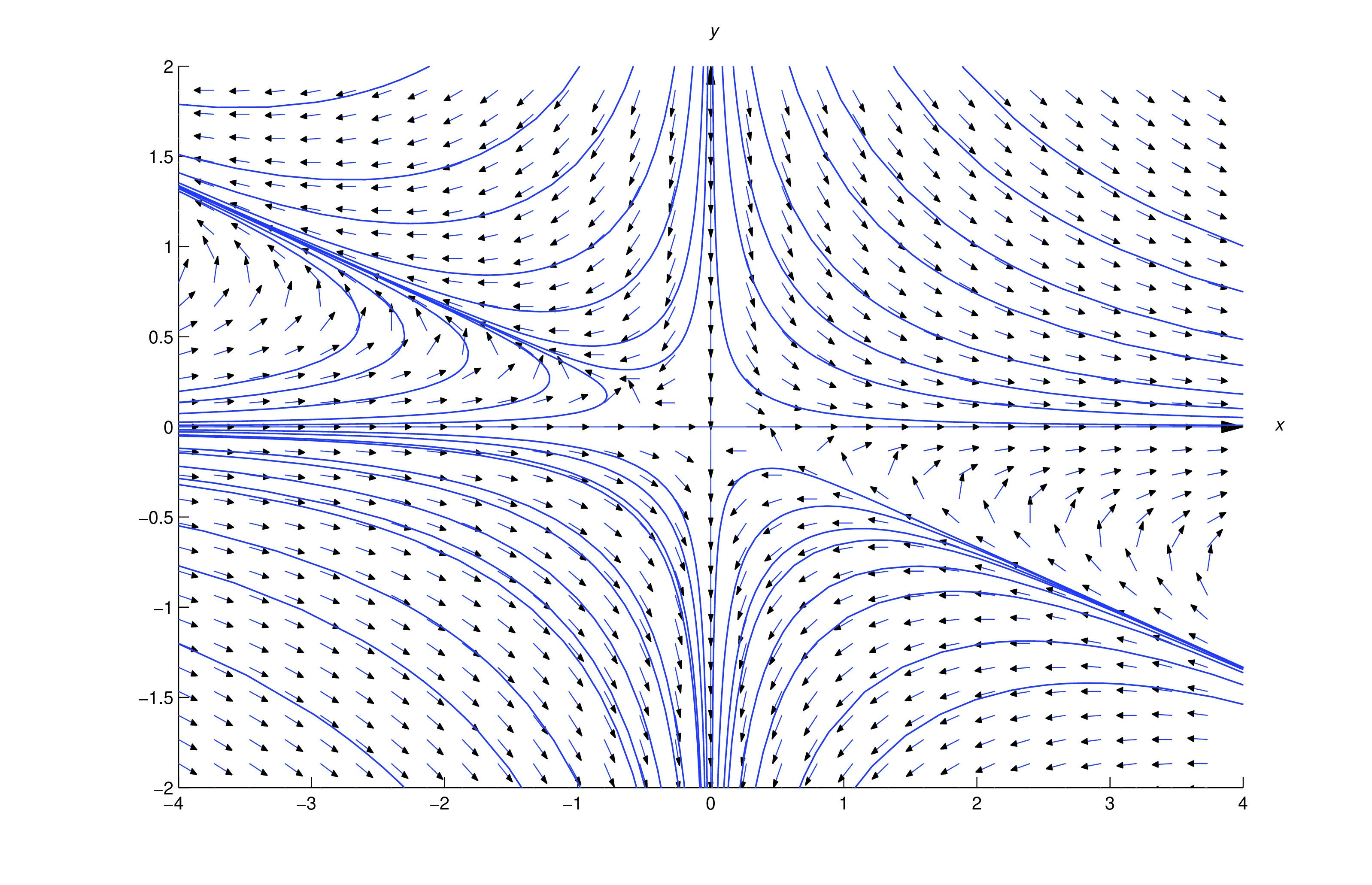
In (eq:2.6.26) and We look for functions and such that that is,
The right side will contain the term if . Then (eq:2.6.28) becomes so . Since and we can take and , which yields the integrating factor . Multiplying (eq:2.6.26) by yields the exact equation We leave it to you to show that this equation has the implicit solution Solving for yields which we rewrite as by renaming the arbitrary constant. This is also a solution of (eq:2.6.26).The figure below shows a direction field and some integral curves for (eq:2.6.26).
Text Source
Trench, William F., ”Elementary Differential Equations” (2013). Faculty Authored and Edited Books & CDs. 8. (CC-BY-NC-SA)