You are about to erase your work on this activity. Are you sure you want to do this?
Updated Version Available
There is an updated version of this activity. If you update to the most recent version of this activity, then your current progress on this activity will be erased. Regardless, your record of completion will remain. How would you like to proceed?
Mathematical Expression Editor
An experiment involving a draining tank.
Tank Draining
This activity is intended to illustrate how the modeling process with differential
equations is used to solve a practical problem. Beginning with physics principles like
conservation of mass and energy and a few simplifying assumptions, a differential
equation is derived to describe the draining of water from a container. After solving
the differential equation, students can predict the time necessary to drain the
container and then check this prediction with a simple experiment using readily
available materials.
Overview of the Model
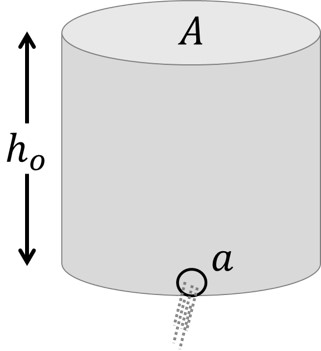
Consider an open cylindrical tank of height that is filled with water or some other
freely flowing liquid. The cross sectional area is a constant value of and a small
circular hole near the bottom has a much smaller area .
When the water is allowed to flow from the hole, the tank will eventually drain until
the water level reaches the hole. Our goal is to predict how long this draining process
will take. We will try to measure the draining time, which we will define as the
elapsed time from when the water is allowed to flow out until the water level reaches
the top of the hole. Before outlining the derivation below, make a prediction about
what parameters impact the draining time. Make a list on paper of every variable
upon which the draining time will depend. Examine your list. Did you include
parameters like air pressure, the density of the fluid, or the shape of the
small hole? Did you include , , and ? If so, what would an increase in these
parameters do to the draining time? As the water drains, will the flow rate remain
constant? Now that you have written down your predictions, let’s derive a model
for this process. When the model is derived, return to your list to check
it.
Before developing a full model, reflect on your physical experience and/or intuition
with draining containers to answer the following question.
Which of the following graphs best predicts how the height of water in this tank will
change with time?
Expand for discussion.
The first option is incorrect. This plot indicates that the height of water is changing
most rapidly in the middle of the draining process and slowly in the beginning and
end. This is not the observed behavior of the height of water in a draining
tank.
The second option is correct. This plot correctly indicates the observed behavior.
Notice that the height of water in the tank changes most rapidly in the
beginning. This is because when the water level is the highest, the flow rate out
will be the greatest. The flow rate out diminishes as the height of water is
reduced.
The third option is incorrect. This plot indicates that the water level will decrease at
a constant rate throughout the draining process. This is not the observed behavior,
because the flow rate of water actually depends on the height of water in the
tank.
The fourth option is incorrect. This plot suggests that the height of water will change
slowly at the beginning and will change more rapidly at the end. This is not the
observed behavior of such a system.
Model Derivation
As with many modeling problems leading to differential equations, it is helpful to
begin with a generic balance equation:
While this principle can be applied to many different quantities for a defined system,
we can immediately apply it to the mass of the water in the tank. This equation can
be called a rate equation because each of the terms refer to a rate (rate of flow in,
rate of destruction, rate of accumulation, etc.) Can you see which of the terms in this
generic equation can be crossed off?
From physics, we recall that mass – just like energy and momentum – is a conserved
quantity under normal circumstances. This means that it cannot be generated or
destroyed. Furthermore, we note that water only flows out of, not into, the tank
during the draining process. This leaves us with:
We also recognize that the density of water (mass per unit volume) is constant.
Thus, since it is easier in our experiment to describe changes in volume and the rate
of flow of volume, we can instead write:
We can now incorporate both of the areas in the diagram above. First, we recognize
that the rate of volume flow out of the tank is equal to the velocity of the water
through the small hole multiplied by the area . Second, we take note of the
relationship between the volume, the height, and the cross sectional area of the
cylindrical tank. The rate of accumulation or depletion of volume is equal to the rate
of change in height multiplied by the cross sectional area. Our balance equation now
becomes:
Observe that the units of this equation are still a rate of change of volume (length
cubed per time). It is helpful that we now have the time rate of change of height in
our equation. We can and will estimate both of the areas. Yet, we do not yet have an
idea of the velocity of the water coming out of the small hole. Our derivation so far
relied on the principle of conservation of mass. To find the velocity out, we
will employ the principle of conservation of energy. For this system, the
principle of conservation of energy leads us to Bernoulli’s Equation, which is an
important relationship between pressure, velocity, and height of a flowing
fluid:
Here, is the pressure, is the density, and is the velocity of the fluid. The
gravitational constant and the height of the fluid, relative to some reference point,
also appear. The units of each term in this equation are pressure, which is force per
unit area. However, it is also helpful to realize that this is also energy per volume.
Can you see this if we note that energy is force times distance and volume is area
times another distance? Bernoulli’s equation shows us how energy, though conserved
overall, can be transferred in different categories. A fluid may have energy due to its
pressure, due to its velocity (kinetic energy), and due to its height (potential energy).
All three of these ways of having energy are included in this equation on a per
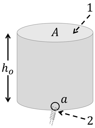
volume basis. Now, considering two points in the system, we can use this
relationship to specify the velocity of water flowing out of the small hole.
Point 1 is at the very top of the water in the tank. Point 2 is on the water as it leaves
the small hole. Bernoulli’s equation is applied to these two points:
Since both points are open to the atmosphere, they are at almost exactly the same
pressure. The small difference in height does not produce a very different air pressure.
For this reason, and can be crossed off together. Since the density of water does not
change at all, it can be cancelled from all of the remaining terms. Rearranging gives
the following:
Further simplification is possible if we neglect . This is defensible because is much
larger than since the cross sectional area of the tank is – in most cases –
significantly larger than the area of the small hole. The square of must therefore be
smaller, relatively speaking, than the square of . Water will be moving much more
quickly out of the small hole than the movement of the top surface of the water. We
can replace the different in heights between two points with , which is the height of
water above the small hole at any point in time. This can now be written
as:
It is evident that as the tank drains, the velocity of the water draining out will
decrease toward zero since the height of the water is decreasing toward zero. When
we conduct the experiment, we expect that the fastest stream of water will be seen at
the very beginning. Having solved for the velocity at Point 2, which is the “velocity
out” in the simplified balance equation above, we can now put everything
together:
Since , , and are all constant in our model of the cylindrical tank, we can lump all
the constants together as and write:
It is instructive to check the units of this differential equation, which are length per
time since it gives us the rate of change of height. Note that the units of the constant
are . We have now derived a differential equation for the height of the fluid in the
tank by using principles from physics and some appropriate simplifications.
Separation and integration leads us to a solution for water height as a function of
time:
Here we specify the constant of integration in terms of the initial height at
.
Rearrangement gives the solution of our differential equation:
From here, we can determine the time necessary for the tank to drain, because this
is when .
If we substitute for the constant , we find that the final time is
Note that, according to our assumptions in this model, no other factors will impact
the draining time: not the air pressure, the density of the fluid, or the shape of the
drain hole. In fact, the drain hole and the cross section of the tank could be circular,
square, or any other shape. We only require that the area of the cross section of the
tank remain constant. For instance, this model would correctly predict the
time to drain a cube shaped container. One other interesting aspect of the
mathematics here is evident when one studies the solution to the differential
equation, which is parabolic in form. Notice that if the time exceeds the
calculated draining time, the solution predicts that the height of the water
would again increase. This is an aphysical (not real) prediction, because once
the tank drains completely the height of the fluid will stay at exactly zero.
Examine the differential equation and note that is a stable (equilibrium)
solution.
Before conducting an experiment to check the accuracy of this model, let’s
examine your predictions of which parameters impact the draining time.
Consider a tank with cross sectional area and hole area with an initial
height . What will happen to the draining time in each of the following
cases?
If is doubled, the draining time will…
Shorten by some amount that cannot be
specifiedShorten by halfRemain unchangedLengthen to twice its initial valueLengthen by some amount that cannot be specifiedChange in some other way
Expand for discussion.
In the equation for above, the draining time is directly proportional to the cross
sectional area of the tank .
If is doubled, the draining time will…
Shorten by some amount that cannot be
specifiedShorten by halfRemain unchangedLengthen to twice its initial valueLengthen by some amount that cannot be specifiedChange in some other way
Expand for discussion.
While a larger initial height will cause the draining time to increase, it is interesting
to note that the dependence is not directly proportional in the same way as it was
with cross sectional area . Doubling the initial height will cause the draining time to
be just over larger. Note that the initial height is inside the square root in the
equation for above.
Tank Draining Experiment
To conduct your own experiment, you should assemble the following near a sink or an
outside location:
(a)
A plastic bottle or other container that has a constant cross section. Most
containers, such as a two-liter soda bottle, would work. Ideally, the bottle
will be at least partially transparent to see the water level. The top should
be open to the atmosphere to prevent a vacuum. You could even choose
to cut the top of the bottle off with scissors to make measuring easier,
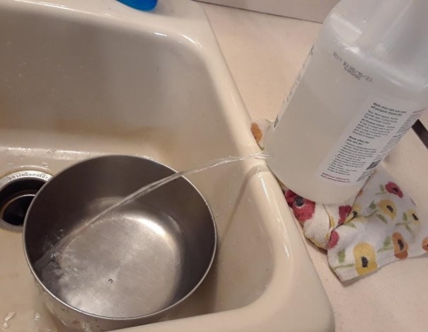
although this is not required. The example demonstrated here is done with
a plastic vinegar bottle shown at right. Note that we will only allow the
water to drain through the region with a constant cross section (just above
the label to the hole punctured just below the label).
(b)
A pushpin that can be used to poke a small hole for the drain.
(c)
A pencil or pen that can be used to widen the drain hole.
(d)
A ruler with fine gradations, preferably with metric units such as
centimeters.
(e)
A stopwatch, clock, or phone to record the drain time
Use the pushpin to start the hole, then widen it with the pencil or pen. Try to
make the whole as close to circular as possible. The diameter of a pen, less
than , is an appropriate size to conduct a first experiment, but you could do
more experiments after incrementally widening the hole. Mark the place on
the bottle for the initial water level. Plan to drain only the region with a
constant cross sectional area. (Our simple model was not derived for an
area A that depended on the height.) Measure this initial height from your
water mark down to the top of the small hole. Also make your best estimate
of the diameter of the container and the small hole in order to calculate
the areas and . If using a container with something other than a circular
cross section, calculate the area according to that geometry. Use all of these
parameters to estimate the time to drain . It is recommended that you convert
all parameters to a common unit such as meters and use . As you fill the
bottle to the line, you could leave the pen stuck in the bottle or keep your
finger over the hole. Make your best estimate of the draining time and stop
the timer the moment the water level reaches the top of the hole. As the
tank drains, recall our prediction that the velocity of the stream would be
largest at the beginning. Draining will slow down greatly as the water height
diminishes.
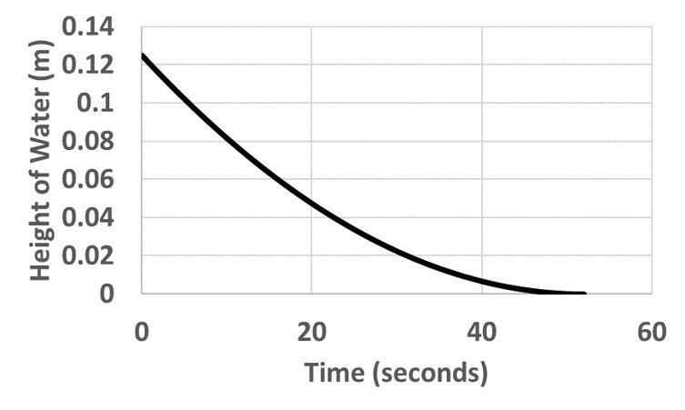
In this example, the initial height was measured to be . The hole diameter was
approximated to be about , giving a hole area . The container diameter was about ,
giving a cross sectional area . Note that is over times larger than , supporting our
previous assumption that is much larger than . The lumped constant is thus
calculated to be and the draining time is predicted to be about seconds. See the
predicted trajectory of the water level vs. time in the plot below. When the
experiment was carried out, it actually took seconds for the tank to drain.
Thus, the observed time was almost longer than the predicted time. This
is not bad. Is your estimate also slightly shorter than the actual draining
time?
Sources of Error
It is instructive to consider what sources of error may have been most important in
our derivation and measurements. List what assumptions you believe may have been
most dubious. Are all of your measurements accurate? Below, we will examine each
major assumption and also estimate possible measurement errors in our analysis.
When possible, we can predict whether a flaw in our model would cause an
overestimate or an underestimate in draining time.
(a)
We assumed that the liquid water was freely flowing. Specifically, we
assumed that the viscosity of our fluid was negligible. One can imagine
the importance of viscosity in the case of less freely flowing substances like
honey or molasses. Furthermore, it is possible that rough edges near our
small drain hole – crudely poked with a pen or pencil – could have inhibited
the flow of water, slightly slowing the draining process. A fluid’s viscosity
causes resistance to flow that – to a certain extent – lessens the overall
conversion of potential to kinetic energy because some of that energy goes
into internal energy (essentially heating the fluid and its surroundings).
In the case of water, it is likely that the velocity flowing out of the tank
was overestimated by a small amount – likely a couple percent. Thus, for
this reason, the model used here would tend to underestimate the draining
time. In our example above, we might have been a bit closer to the correct
answer.
(b)
Neglecting the term seemed reasonable during the derivation, and allowed
us to further simplify Bernoulli’s Equation:
Instead of neglecting this velocity of the top surface of the water, we could
have chosen to relate it to the other velocity of the water at the drain hole.
Recall that our balance equation had led to the following relationship:
We recognize that the ”velocity out” is and that is equal to , since it is
the rate of change of the height of the water. For that reason, we recognize
that . This enables us to write Bernoulli’s equation as:
In contrast to our previous simplified result , we now arrive at:
However, here we realize that our previous simplification was more than
warranted. As noted in the example above, the area is more than three
hundred times smaller than , which means that denominator is very
nearly , making the difference negligible. Other assumptions and errors in
measurement likely dwarf this error.
(c)
Measurement error may also have been significant. For instance, we
measured the small drain hole with a ruler, approximating the diameter
to be about . Given its small size, this is a difficult estimate to make
with only a ruler. Run the calculation again to see that if we had been
just off in this estimate of this diameter, the draining time would vary
by almost , or about seconds. This is a substantial change in the overall
prediction resulting from a very modest difference in our measurement.
Other measurement errors are possible including the other two lengths
and the recorded time, but these are likely smaller than that caused by
the measurement of the small hole. This suggests that the accuracy of
our modeling is highly dependent on the estimation of key distances, and
measurement errors here could outweigh the effects of our assumptions
regarding the physics of the model. Measurement with calipers or the
careful use of a drill bit to make the drain hole may be warranted to
improve the accuracy of the model.