We begin our study of Laplace transforms with the definition, and we derive the Laplace Transform of some basic functions.
Introduction to the Laplace Transform
Definition of the Laplace Transform
To define the Laplace transform, we first recall the definition of an improper integral. If is integrable over the interval for every , then the improper integral of over is defined as
We say that the improper integral converges if the limit in (eq:8.1.1) exists; otherwise, we say that the improper integral diverges or does not exist. Here’s the definition of the Laplace transform of a function .It is important to keep in mind that the variable of integration in (eq:8.1.2) is , while is a parameter independent of . We use as the independent variable for because in applications the Laplace transform is usually applied to functions of time.
The Laplace transform can be viewed as an operator that transforms the function into the function . Thus, (eq:8.1.2) can be expressed as The functions and form a transform pair, which we’ll sometimes denote by It can be shown that if is defined for then it’s defined for all .
Computation of Some Simple Laplace Transforms
Tables of Laplace transforms
Extensive tables of Laplace transforms have been compiled and are commonly used in applications. The brief table of Laplace transforms in Trench 8.8 will be adequate for our purposes.
We’ll sometimes write Laplace transforms of specific functions without explicitly stating how they are obtained. In such cases you should refer to the table of Laplace transforms.
Linearity of the Laplace Transform
The next theorem presents an important property of the Laplace transform.
- Proof
- We give the proof for the case where . If then
The First Shifting Theorem
The next theorem enables us to start with known transform pairs and derive others.
Existence of Laplace Transforms
Not every function has a Laplace transform. For example, it can be shown that for every real number . Hence, the function does not have a Laplace transform.
Our next objective is to establish conditions that ensure the existence of the Laplace transform of a function. We first review some relevant definitions from calculus.
Recall that a limit exists if and only if the one-sided limits both exist and are equal; in this case, Recall also that is continuous at a point in an open interval if and only if which is equivalent to
For simplicity, we define so (eq:8.1.12) can be expressed as If and have finite but distinct values, we say that has a jump discontinuity at , and is called the jump in at the figure below.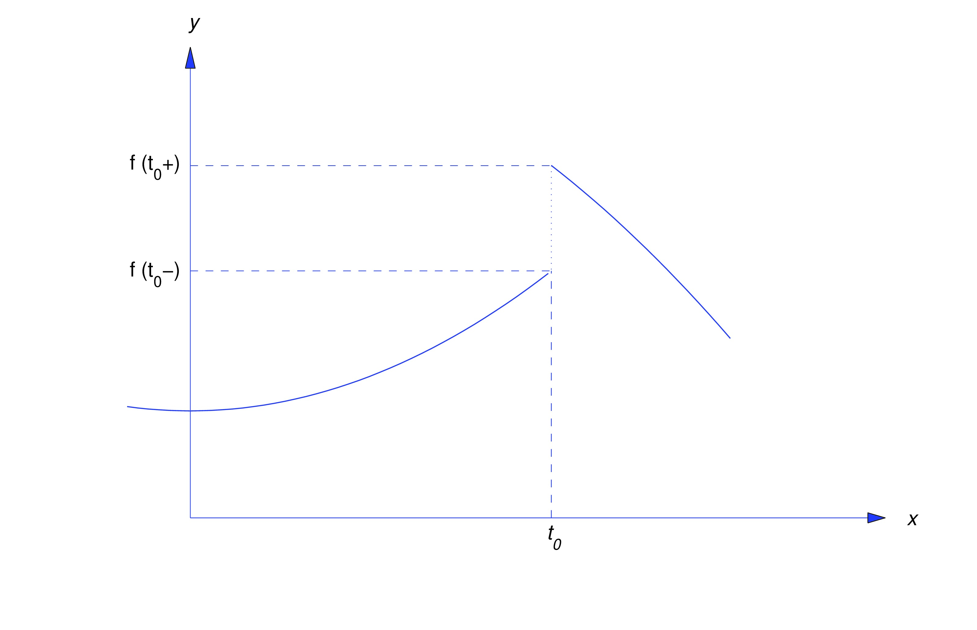
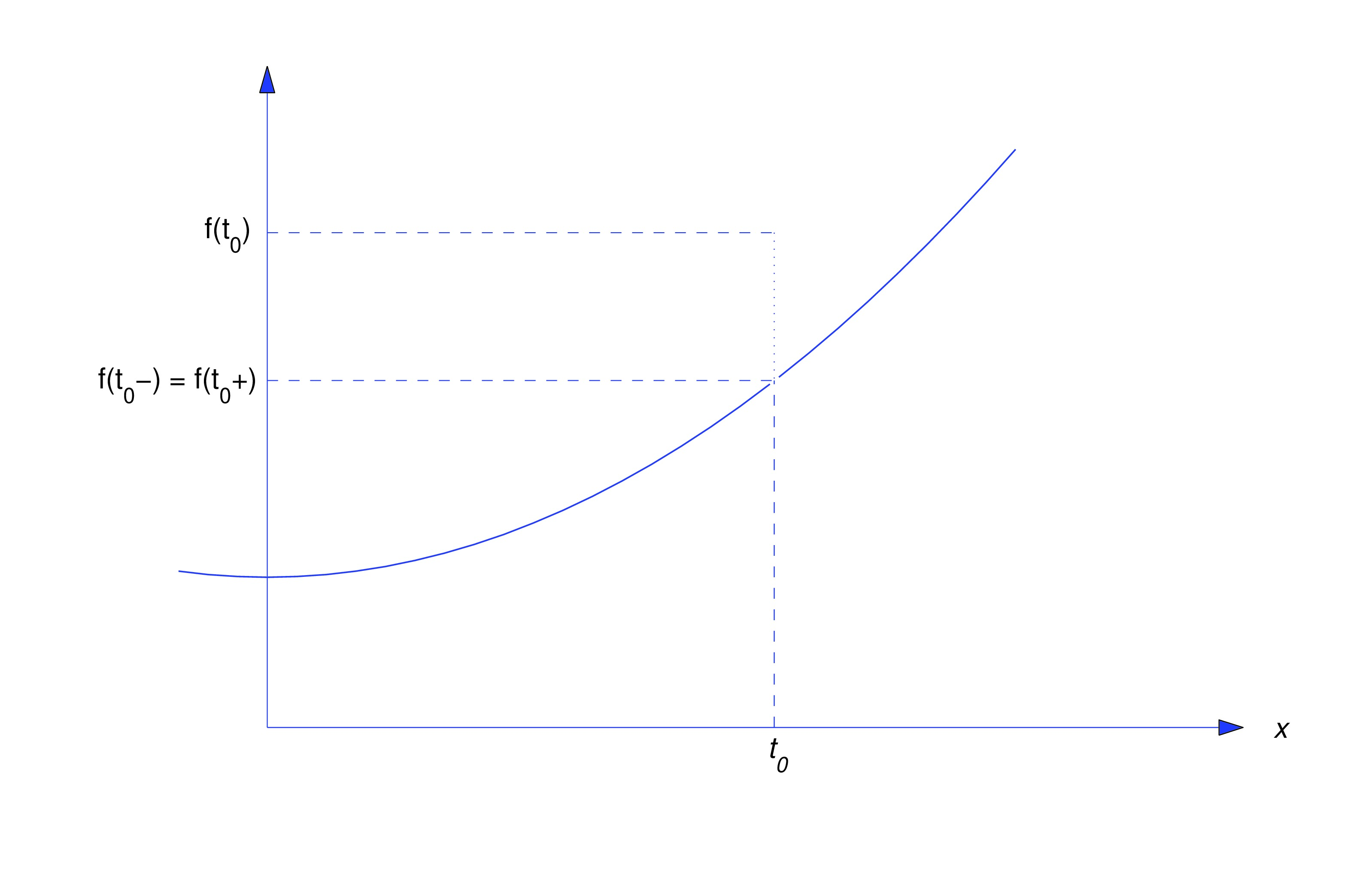
If and are finite and equal, but either isn’t defined at or it’s defined but we say that has a removable discontinuity at (see the figure below).This terminology is appropriate since a function with a removable discontinuity at can be made continuous at by defining (or redefining)
- (a)
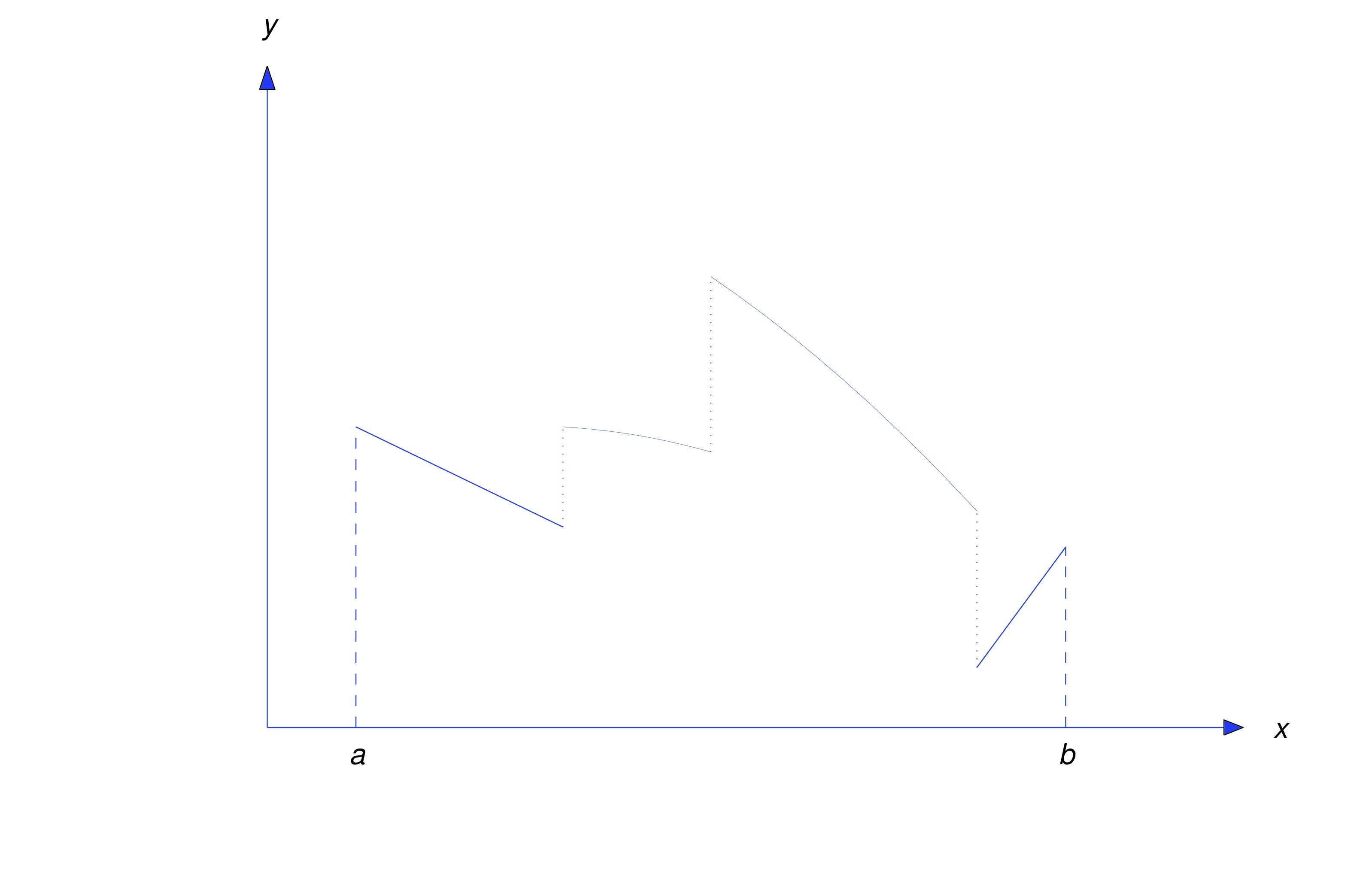
- A function is said to be piecewise continuous on a finite closed interval if and are finite and is continuous on the open interval except possibly at finitely many points, where may have jump discontinuities or removable discontinuities.
- (b)
- A function is said to be piecewise continuous on the infinite interval if it’s piecewise continuous on for every .
The figure below shows the graph of a typical piecewise continuous function.
It is shown in calculus that if a function is piecewise continuous on a finite closed interval then it’s integrable on that interval. But if is piecewise continuous on , then so is , and therefore exists for every . However, piecewise continuity alone does not guarantee that the improper integral
converges for in some interval . For example, we noted earlier that (eq:8.1.13) diverges for all if . Stated informally, this occurs because increases too rapidly as . The next definition provides a constraint on the growth of a function that guarantees convergence of its Laplace transform for in some interval .The next theorem gives useful sufficient conditions for a function to have a Laplace transform.
Text Source
Trench, William F., ”Elementary Differential Equations” (2013). Faculty Authored and Edited Books & CDs. 8. (CC-BY-NC-SA)