We study a number of ways that families of curves can be defined using differential equations.
Applications to Curves
One-Parameter Families of Curves
We begin with two examples of families of curves generated by varying a parameter over a set of real numbers.
Equations (eq:4.5.1) and (eq:4.5.2) define one–parameter families of curves. (Although (eq:4.5.2) isn’t in the form (eq:4.5.3), it can be written in this form as .)
Recall from Trench 1.2 that the graph of a solution of a differential equation is called an integral curve of the equation. Solving a first order differential equation usually produces a one–parameter family of integral curves of the equation. Here we are interested in the converse problem: given a one–parameter family of curves, is there a first order differential equation for which every member of the family is an integral curve. This suggests the next definition.
To find a differential equation for a one–parameter family we differentiate its defining equation (eq:4.5.5) implicitly with respect to , to obtain
If this equation doesn’t, then it’s a differential equation for the family. If it does contain , it may be possible to obtain a differential equation for the family by eliminating between (eq:4.5.5) and (eq:4.5.7).The next example shows that members of a given family of curves may be obtained by joining integral curves for more than one differential equation.
- (a)
- Try to find a differential equation for the family of lines tangent to the parabola .
- (b)
- Find two tangent lines to the parabola that pass through , and find the points of tangency.
Differentiating (eq:4.5.10) with respect to yields We can express in terms of and by rewriting (eq:4.5.10) as and using the quadratic formula to obtain
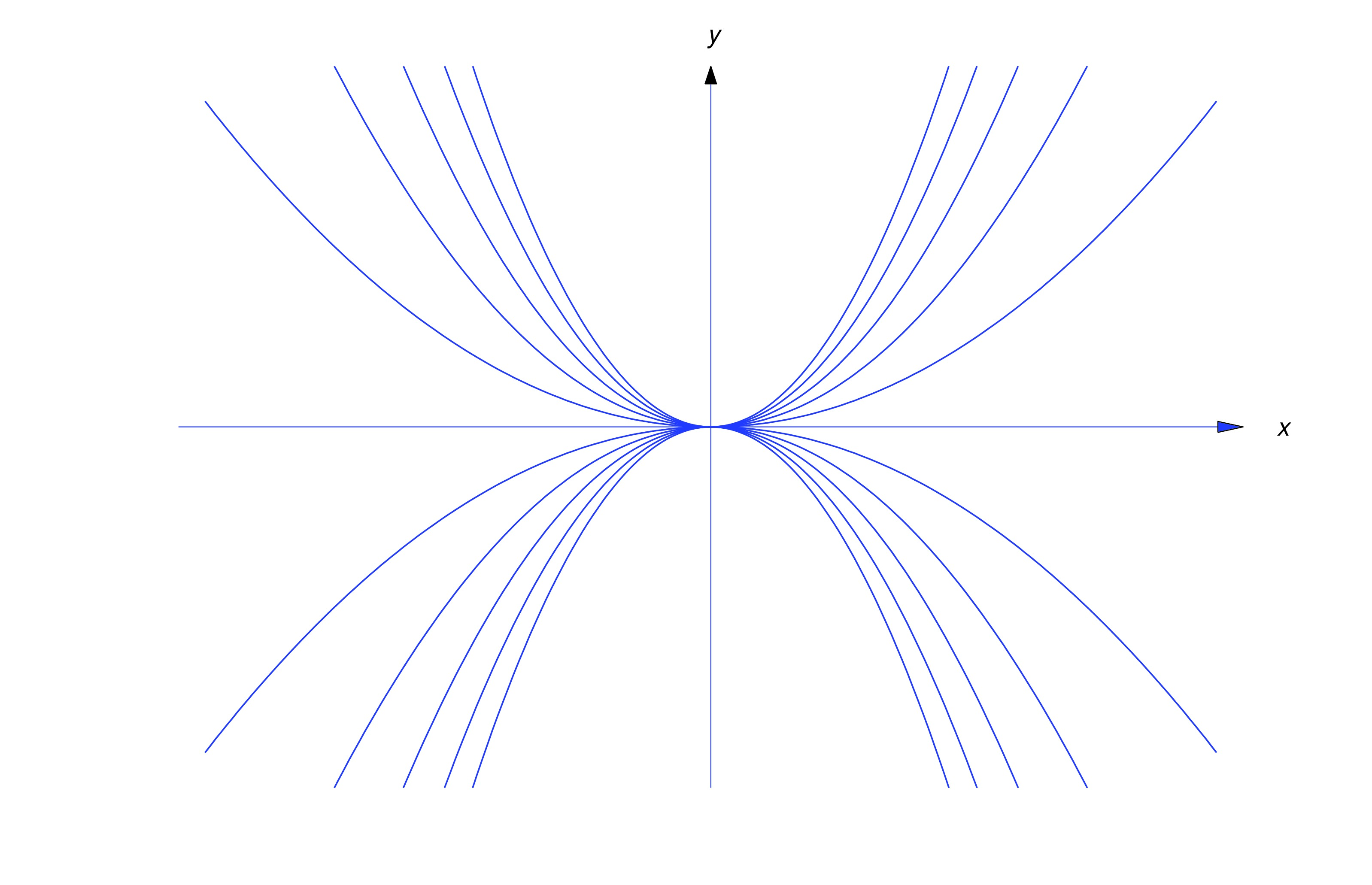
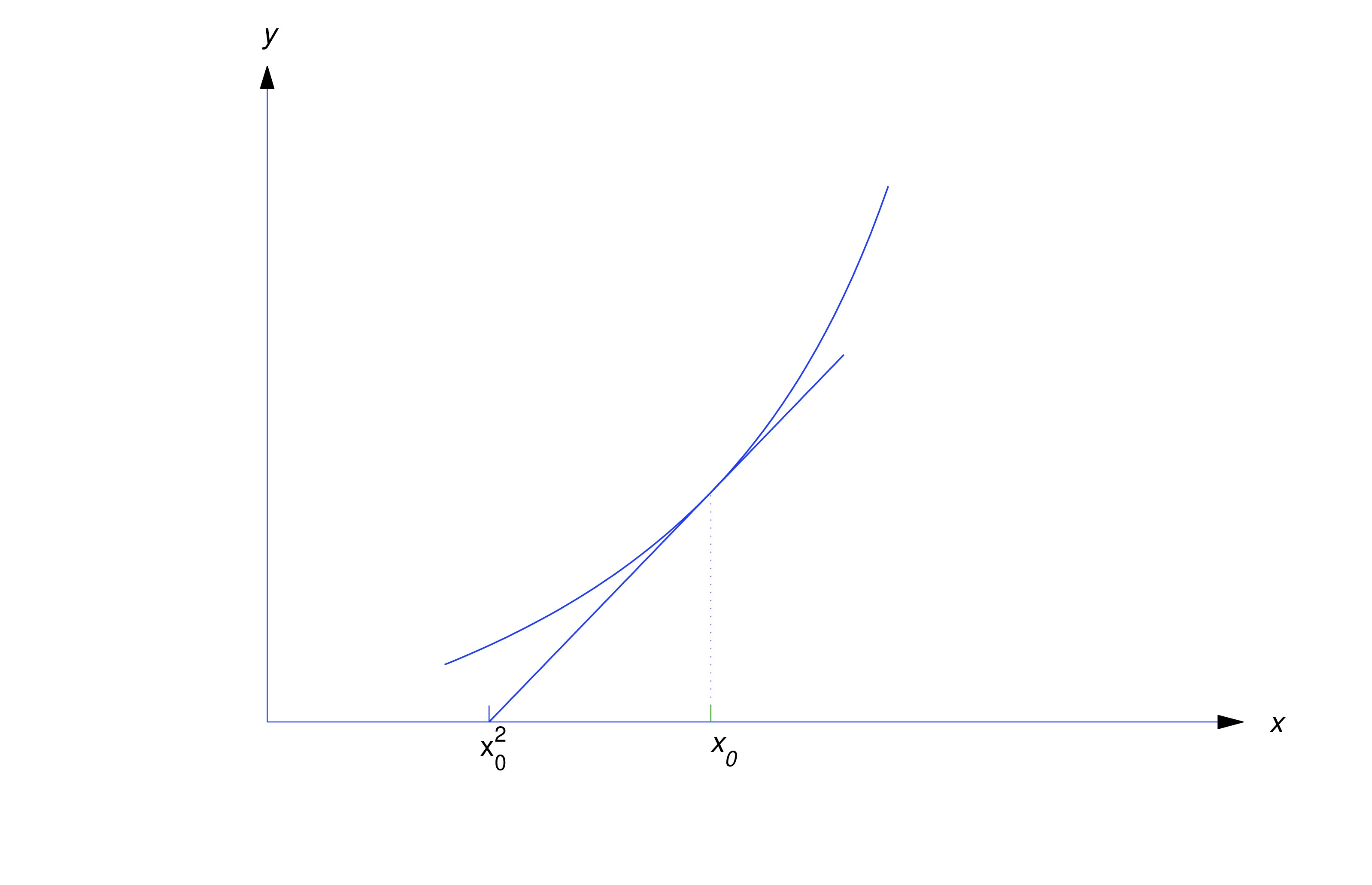
We must choose the plus sign in (eq:4.5.11) if and the minus sign if ; thus, and Since , this implies that and Neither (eq:4.5.12) nor (eq:4.5.13) is a differential equation for the family of tangent lines to the parabola . However, if each tangent line is regarded as consisting of two tangent half lines joined at the point of tangency, (eq:4.5.12) is a differential equation for the family of tangent half lines on which is less than the abscissa of the point of tangency (See figure below).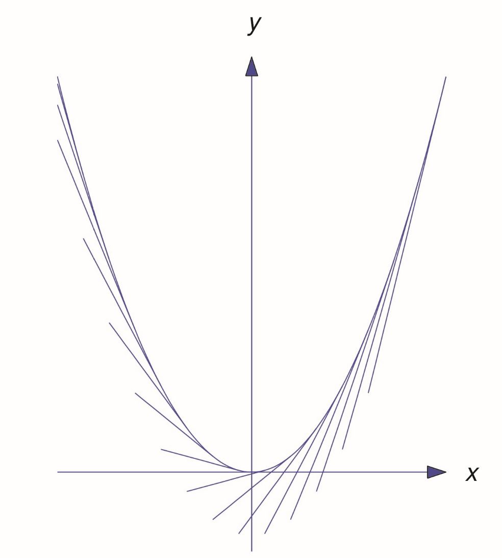
Equation (eq:4.5.13) is a differential equation for the family of tangent half lines on which is greater than this abscissa (See figure below).
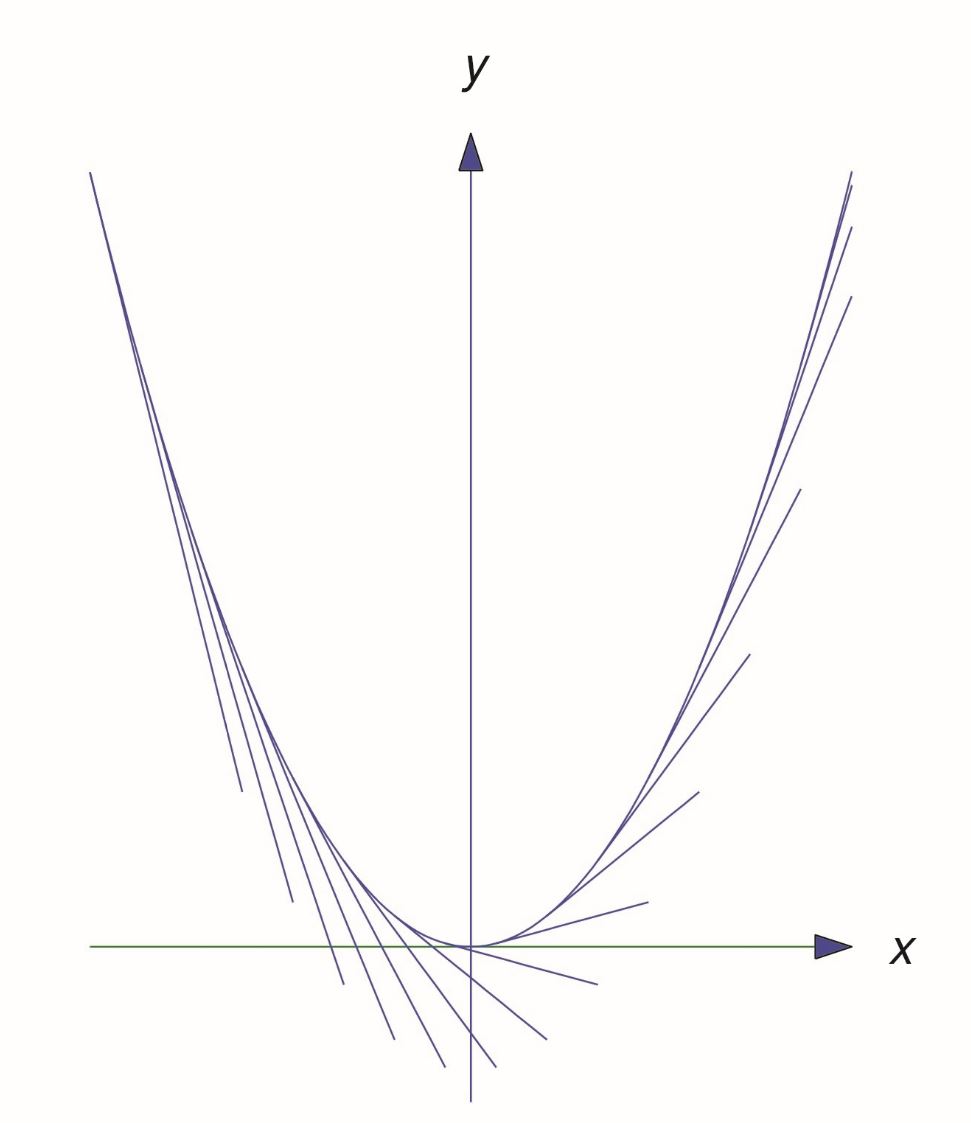
The parabola is also an integral curve of both (eq:4.5.12) and (eq:4.5.13).
item:4.5.6b From (eq:4.5.10) the point is on the tangent line through if and only if which is equivalent to Letting in (eq:4.5.10) shows that is on the line which is tangent to the parabola at , as shown below.
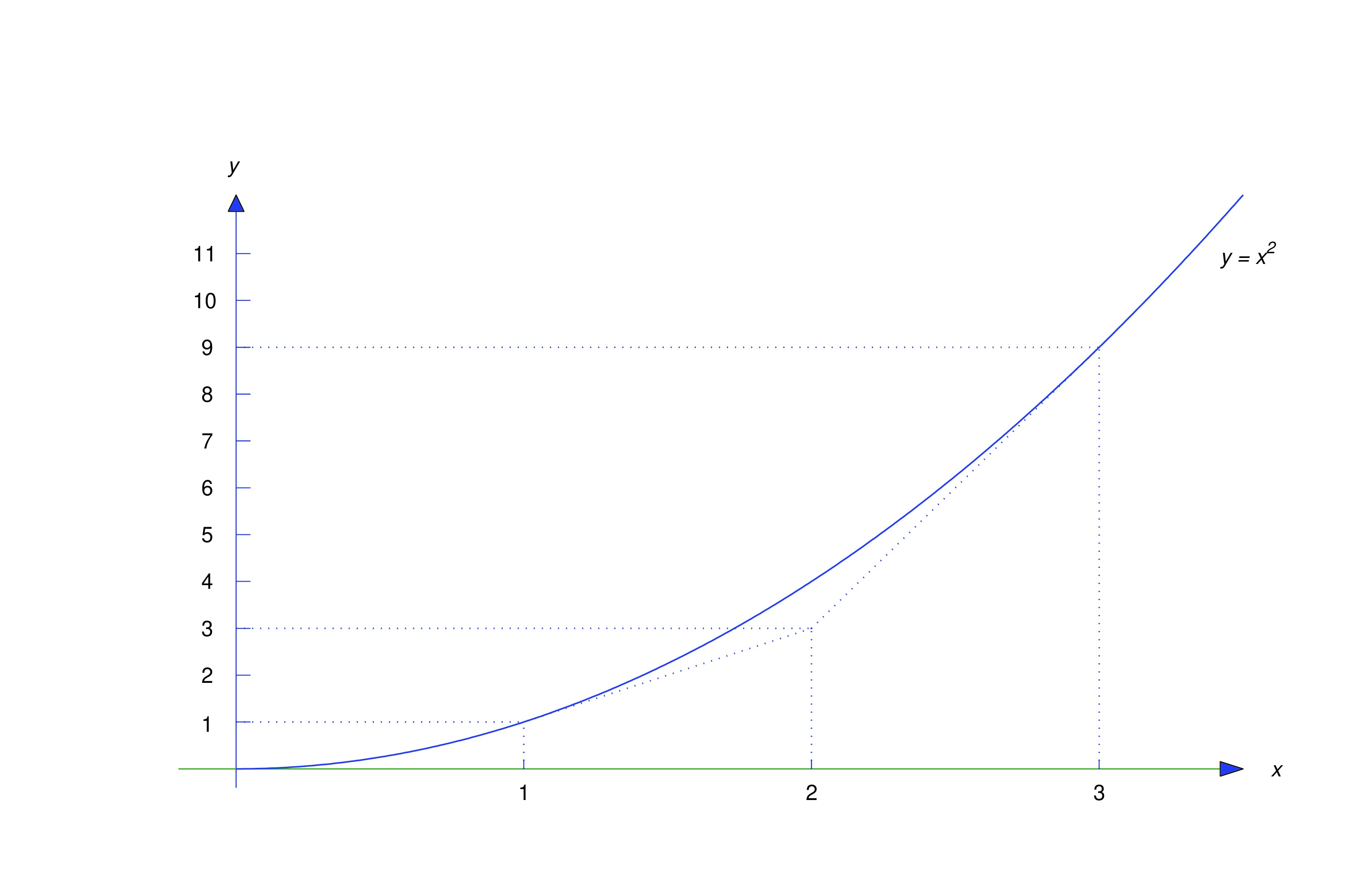
Letting in (eq:4.5.10) shows that is on the line which is tangent to the parabola at , as shown above.
Geometric Problems
We now consider some geometric problems that can be solved by means of differential equations.
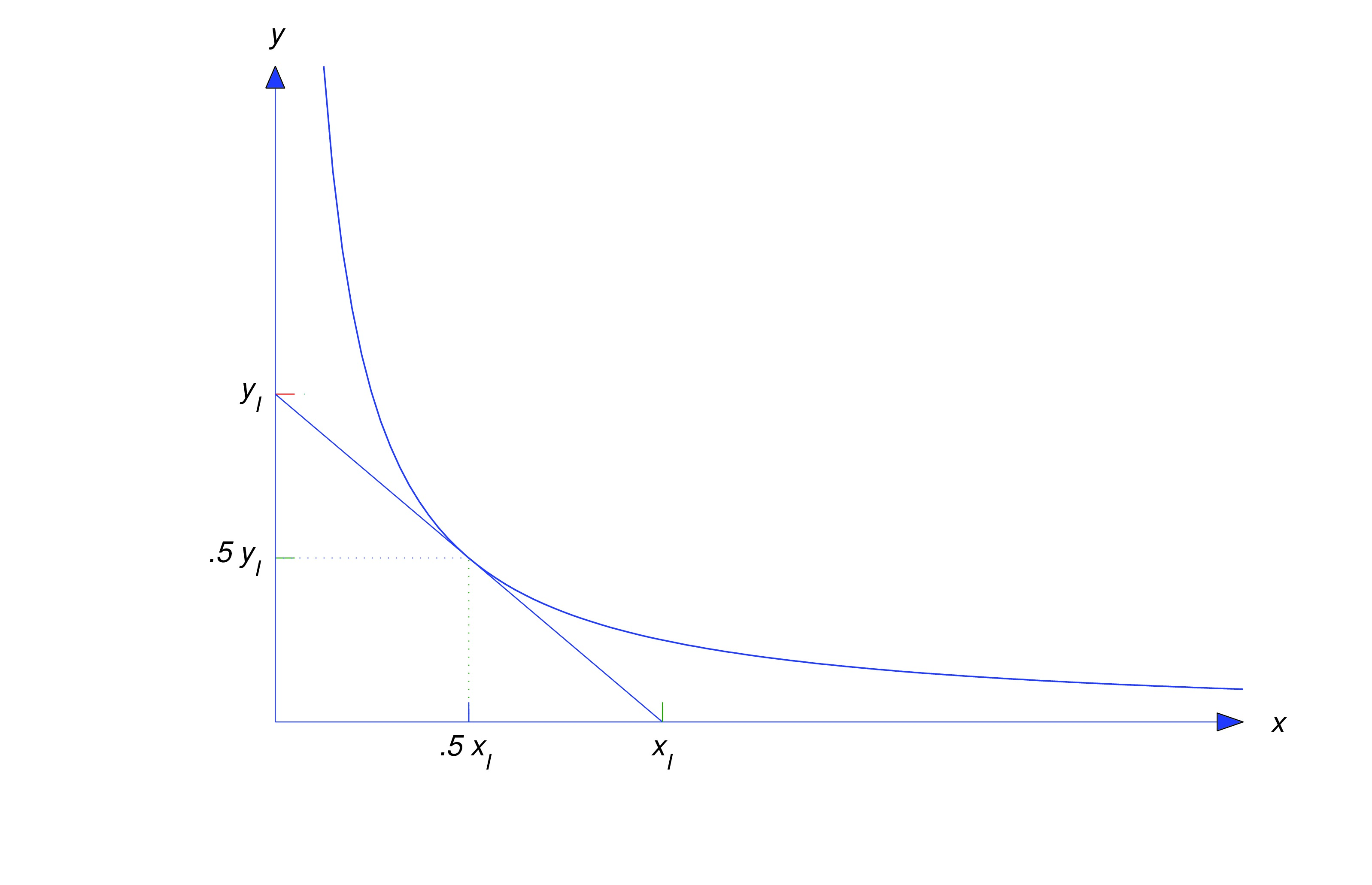
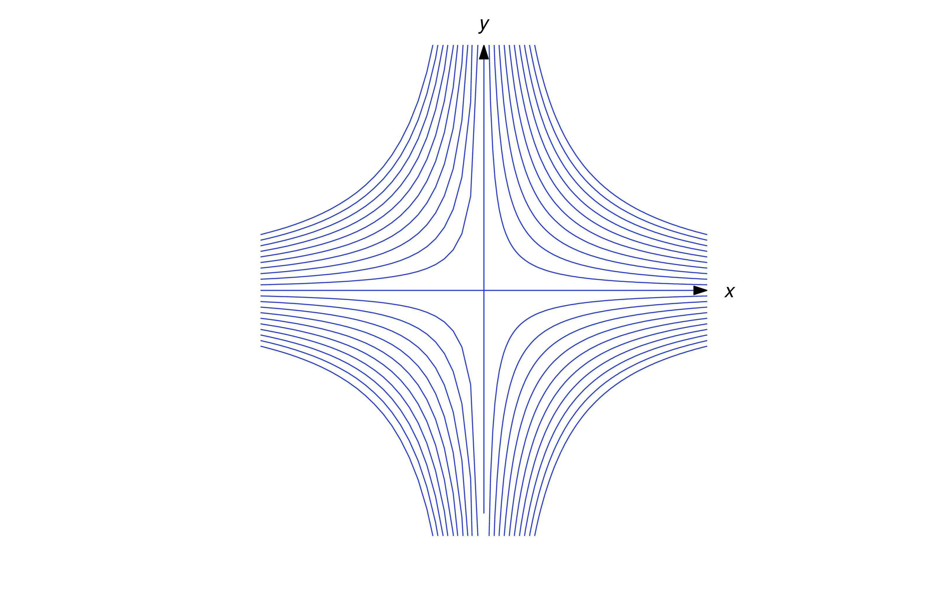
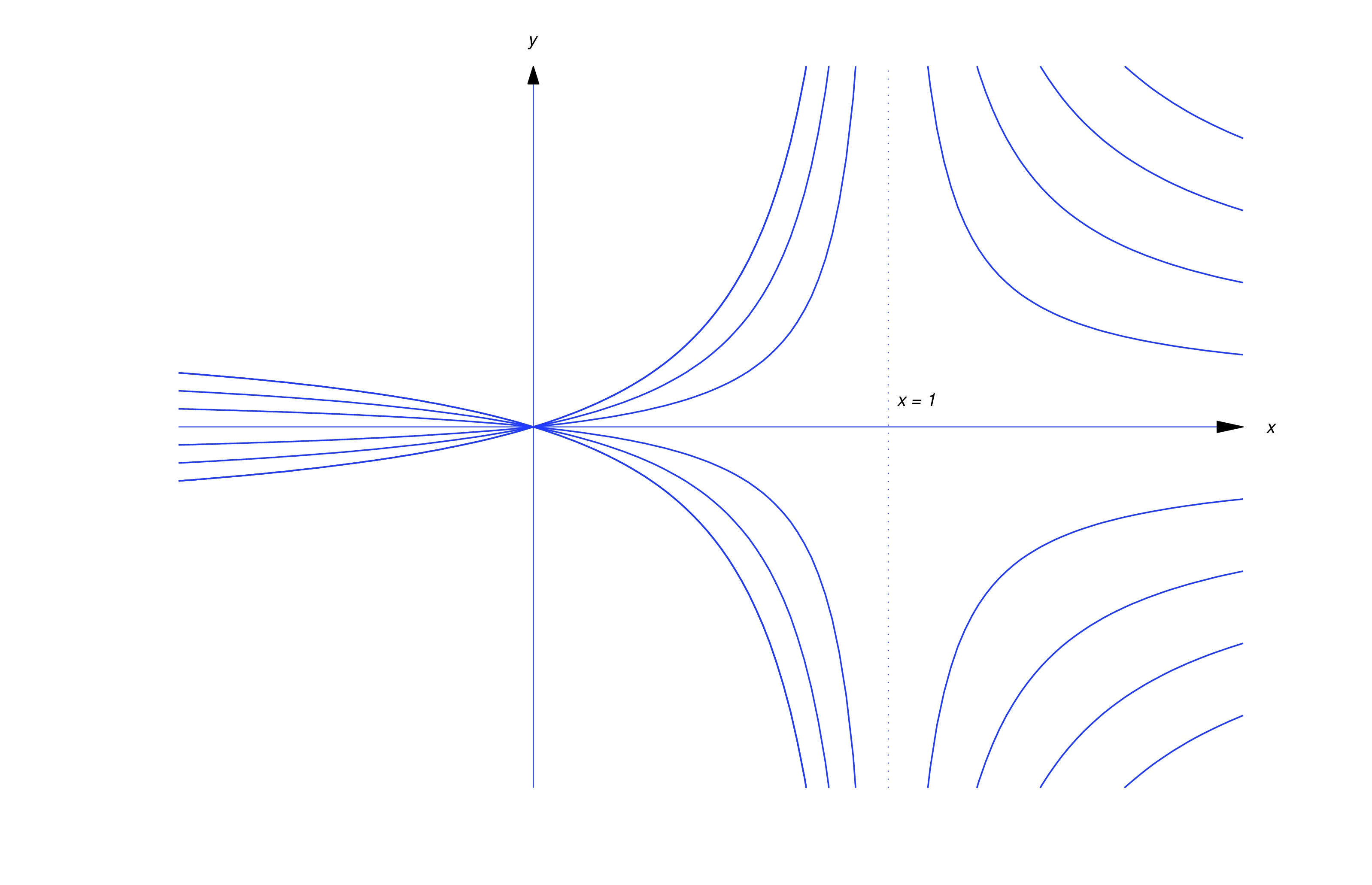
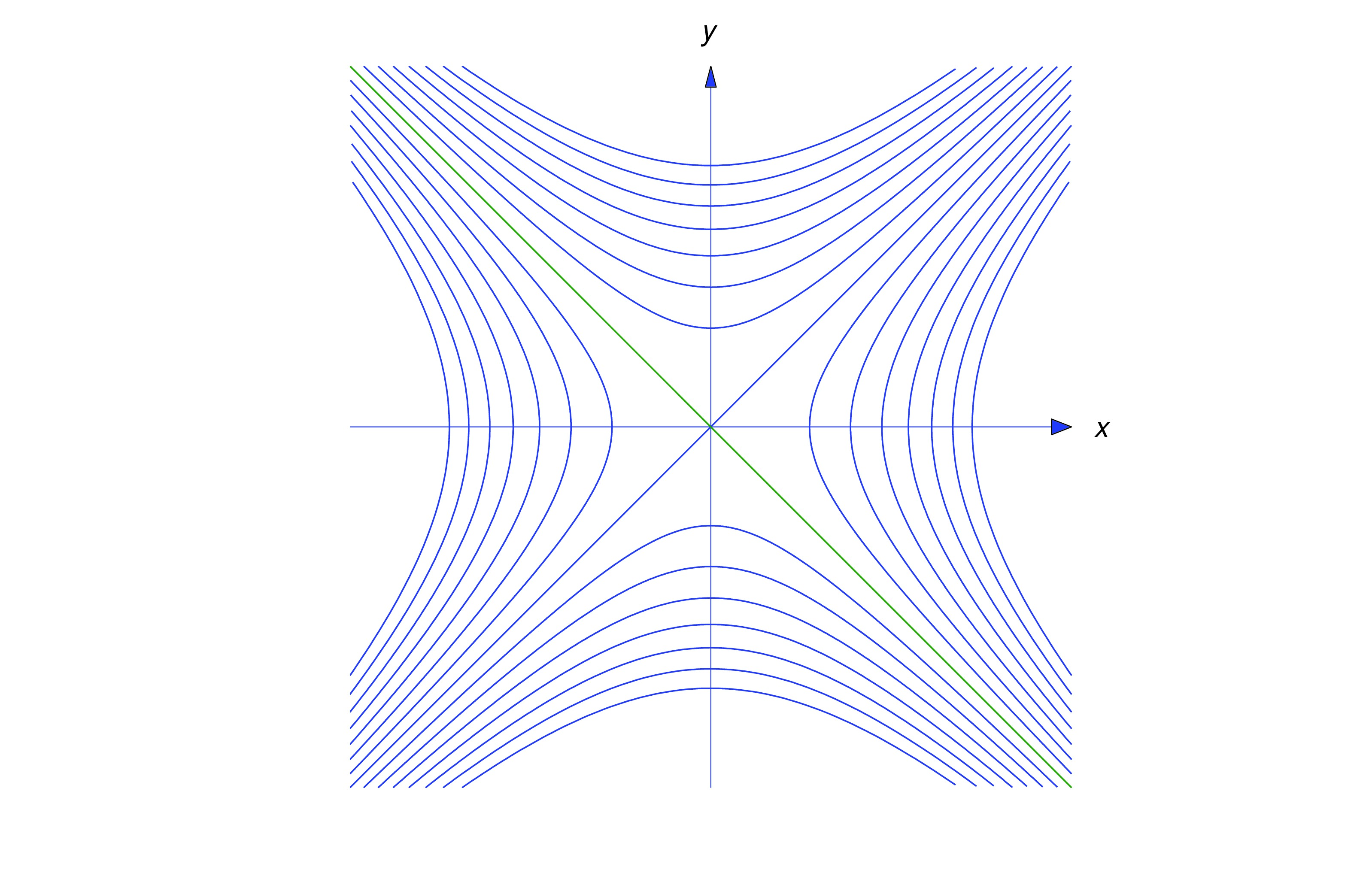
Referring to the figure, we can see that, is the midpoint of the line segment connecting and if and only if and . Substituting the first of these conditions into (eq:4.5.14) or the second into (eq:4.5.15) yields Since is arbitrary we drop the subscript and conclude that satisfies which can be rewritten as Integrating yields , or If this curve is the line , which does not satisfy the geometric requirements imposed by the problem; thus, , and the solutions define a family of hyperbolas, as shown below.
The following interactive will allow you to explore a family of curves with an interesting property. To explore, change the values of and . What do you observe about the relationship between the -coordinate of the point of tangency and the -intercept of the tangent line?
The following example shows how to find a family of solutions that posses the property you observed.
Orthogonal Trajectories
Two curves and are said to be orthogonal at a point of intersection if they have perpendicular tangents at . (See figure below).
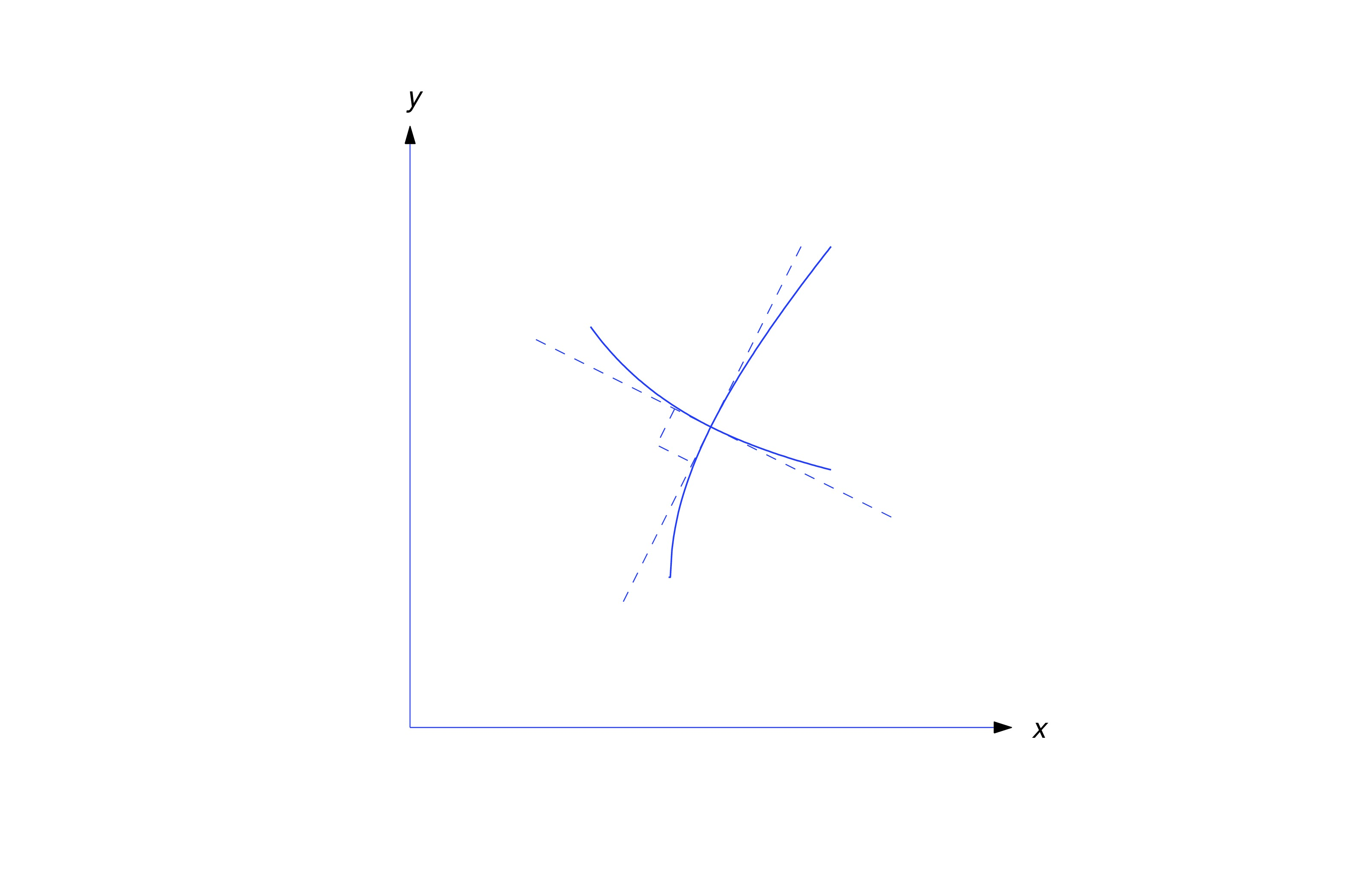
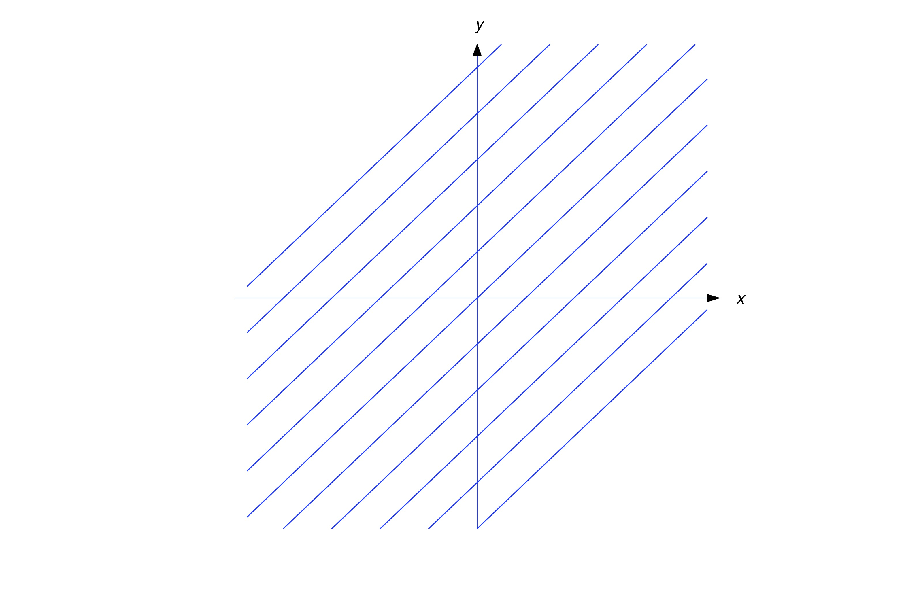
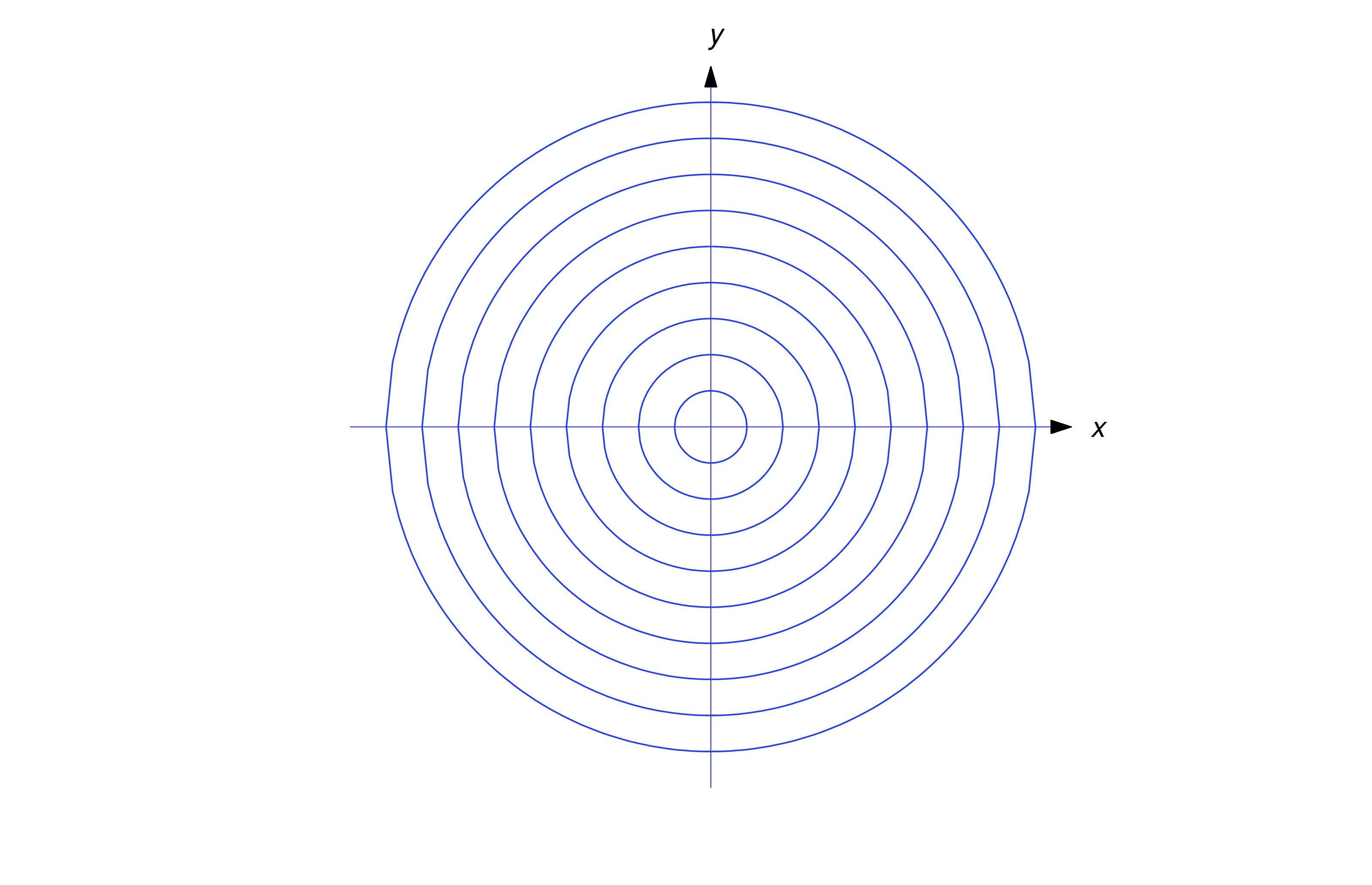
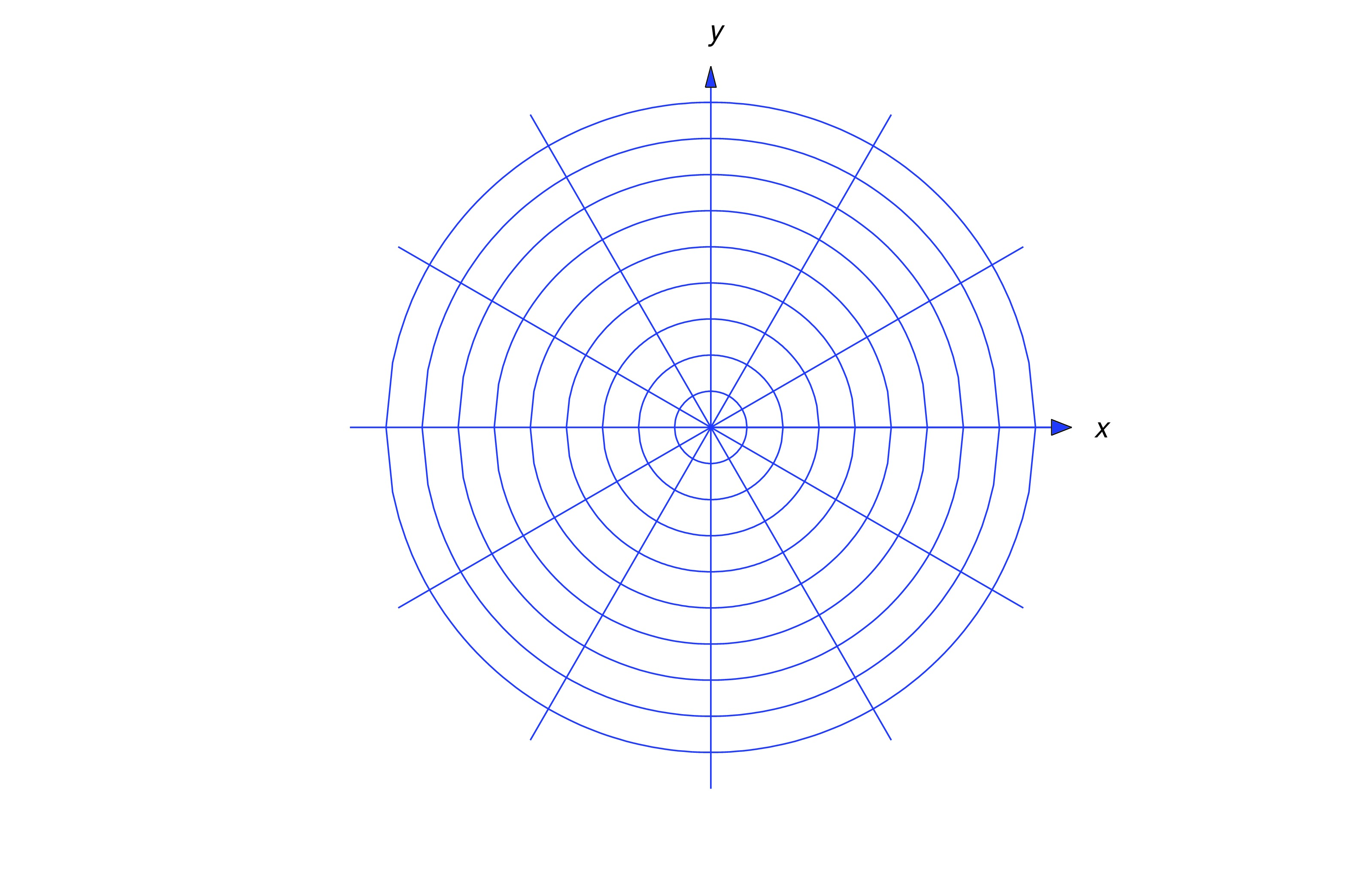
A curve is said to be an orthogonal trajectory of a given family of curves if it’s orthogonal to every curve in the family. For example, every line through the origin is an orthogonal trajectory of the family of circles centered at the origin. Conversely, any such circle is an orthogonal trajectory of the family of lines through the origin.
Orthogonal trajectories occur in many physical applications. For example, if is the temperature at a point , the curves defined by
are called isothermal curves. The orthogonal trajectories of this family are called heat-flow lines, because at any given point the direction of maximum heat flow is perpendicular to the isothermal through the point. If represents the potential energy of an object moving under a force that depends upon , the curves (eq:4.5.16) are called equipotentials, and the orthogonal trajectories are called lines of force.From analytic geometry we know that two nonvertical lines and with slopes and , respectively, are perpendicular if and only if ; therefore, the integral curves of the differential equation are orthogonal trajectories of the integral curves of the differential equation because at any point where curves from the two families intersect the slopes of the respective tangent lines are
This suggests a method for finding orthogonal trajectories of a family of integral curves of a first order equation.
Step 1. Find a differential equation for the given family.
Step 2.
Solve the differential equation to find the orthogonal trajectories.
This is consistent with the theorem of plane geometry which states that a diameter of a circle and a tangent line to the circle at the end of the diameter are perpendicular.
Use the interactive below to visualize the interaction between the family of hyperbolas and the orthogonal trajectories.
When , there are some “nice” solutions with integral coordinates for certain values of . Use the interactive to find them.
The following dynamic interactive will help you visualize the curves.
Text Source
Trench, William F., ”Elementary Differential Equations” (2013). Faculty Authored and Edited Books & CDs. 8. (CC-BY-NC-SA)