We continue our study of constant coefficient homogeneous systems. In this section we consider the case where has real eigenvalues, but does not have linearly independent eigenvectors.
Constant Coefficient Homogeneous Systems II
We saw in Trench 10.4 that if an constant matrix has real eigenvalues (which need not be distinct) with associated linearly independent eigenvectors , then the general solution of is In this section we consider the case where has real eigenvalues, but does not have linearly independent eigenvectors. It is shown in linear algebra that this occurs if and only if has at least one eigenvalue of multiplicity such that the associated eigenspace has dimension less than . In this case is said to be defective. Since it’s beyond the scope of this book to give a complete analysis of systems with defective coefficient matrices, we will restrict our attention to some commonly occurring special cases.
From Example example:10.5.1, we know that all scalar multiples of are solutions of (eq:10.5.1); however, to find the general solution we must find a second solution such that is linearly independent. Based on your recollection of the procedure for solving a constant coefficient scalar equation in the case where the characteristic polynomial has a repeated root, you might expect to obtain a second solution of (eq:10.5.1) by multiplying the first solution by . However, this yields , which doesn’t work, since
The next theorem shows what to do in this situation.
A complete proof of this theorem is beyond the scope of this book. The difficulty is in proving that there’s a vector satisfying (eq:10.5.2), since . We’ll take this without proof and verify the other assertions of the theorem.
We already know that in (eq:10.5.3) is a solution of . To see that is also a solution, we compute
To see that and are linearly independent, suppose and are constants such that
We must show that . Multiplying (eq:10.5.4) by shows that By differentiating this with respect to , we see that , which implies , because . Substituting into (eq:10.5.5) yields , which implies that , again becauseNote that choosing the arbitrary constant to be nonzero is equivalent to adding a scalar multiple of to the second solution .
Eigenvectors associated with must satisfy . The augmented matrix of this system is which is row equivalent to Hence, and , where is arbitrary. Choosing yields the eigenvector Therefore is a solution of (eq:10.5.7).
Eigenvectors associated with satisfy . The augmented matrix of this system is which is row equivalent to Hence, and , where is arbitrary. Choosing yields the eigenvector so is a solution of (eq:10.5.7).
Since all the eigenvectors of associated with are multiples of , we must now use Theorem thmtype:10.5.1 to find a third solution of (eq:10.5.7) in the form
where is a solution of . The augmented matrix of this system is which is row equivalent to Hence, and , where is arbitrary. Choosing yields and substituting this into (eq:10.5.8) yields the solution of (eq:10.5.7).Since the Wronskian of at is is a fundamental set of solutions of (eq:10.5.7). Therefore the general solution of (eq:10.5.7) is
Again, it’s beyond the scope of this book to prove that there are vectors and that satisfy (eq:10.5.9) and (eq:10.5.10). Theorem thmtype:10.5.1 implies that and are solutions of . We leave the rest of the proof to you.
We now find a second solution of (eq:10.5.11) in the form where satisfies . The augmented matrix of this system is which is row equivalent to Letting yields and ; hence, and is a solution of (eq:10.5.11).
We now find a third solution of (eq:10.5.11) in the form where satisfies . The augmented matrix of this system is which is row equivalent to Letting yields and ; hence, Therefore is a solution of (eq:10.5.11). Since , , and are linearly independent by Theorem thmtype:10.5.2, they form a fundamental set of solutions of (eq:10.5.11). Therefore the general solution of (eq:10.5.11) is
We omit the proof of this theorem.
To find a third linearly independent solution of (eq:10.5.15), we must find constants and (not both zero) such that the system
has a solution . The augmented matrix of this system is which is row equivalent to Therefore (eq:10.5.17) has a solution if and only if , where is arbitrary. If then (eq:10.5.12) and (eq:10.5.16) yield and the augmented matrix (eq:10.5.18) becomes This implies that , while and are arbitrary. Choosing yields Therefore (eq:10.5.14) implies thatis a solution of (eq:10.5.15). Since , , and are linearly independent by Theorem thmtype:10.5.3, they form a fundamental set of solutions for (eq:10.5.15). Therefore the general solution of (eq:10.5.15) is
Geometric Properties of Solutions when
We’ll now consider the geometric properties of solutions of a constant coefficient system
under the assumptions of this section; that is, when the matrix has a repeated eigenvalue and the associated eigenspace is one-dimensional. In this case we know from Theorem thmtype:10.5.1 that the general solution of (eq:10.5.19) is where is an eigenvector of and is any one of the infinitely many solutions of We assume that .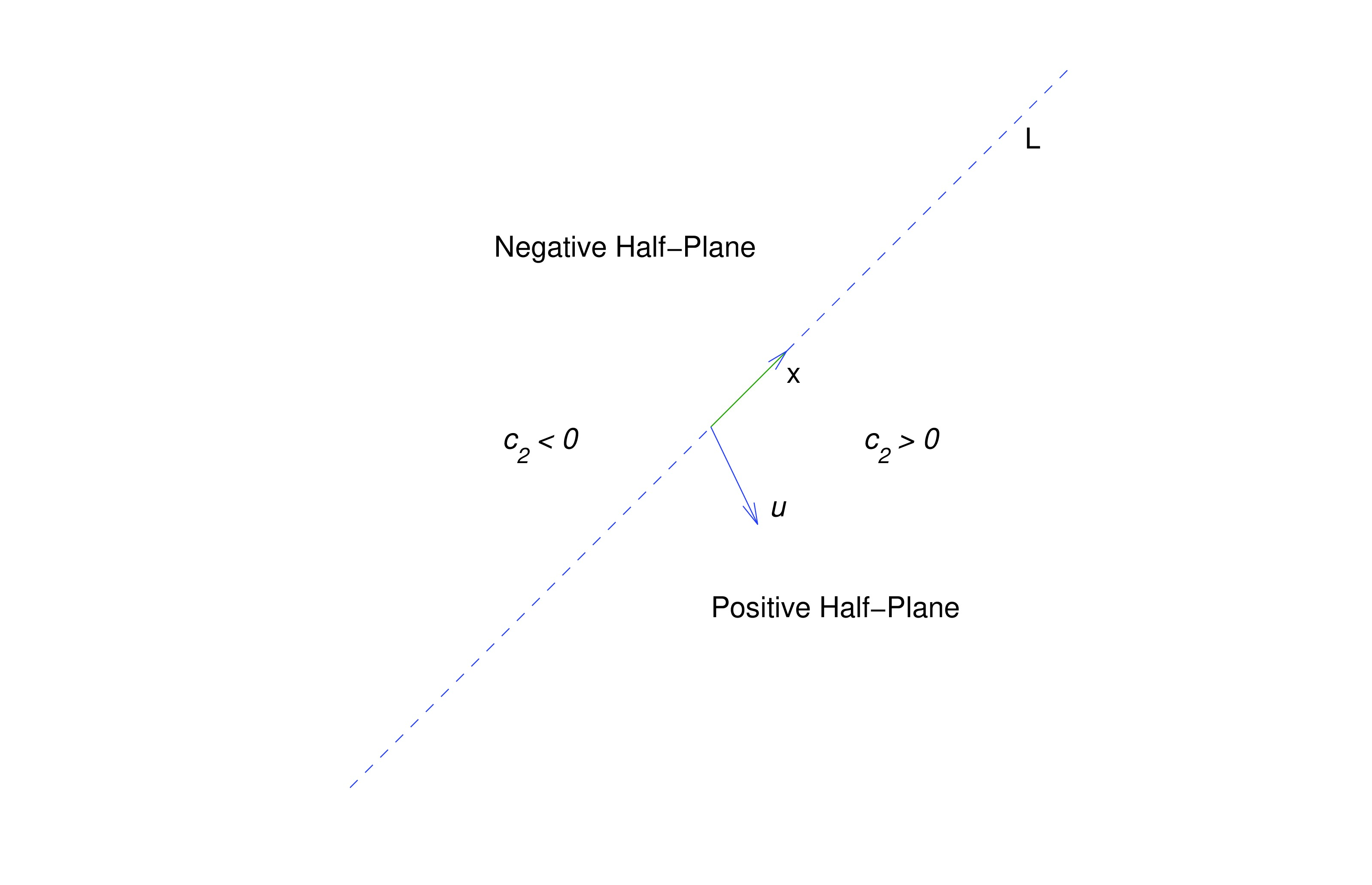
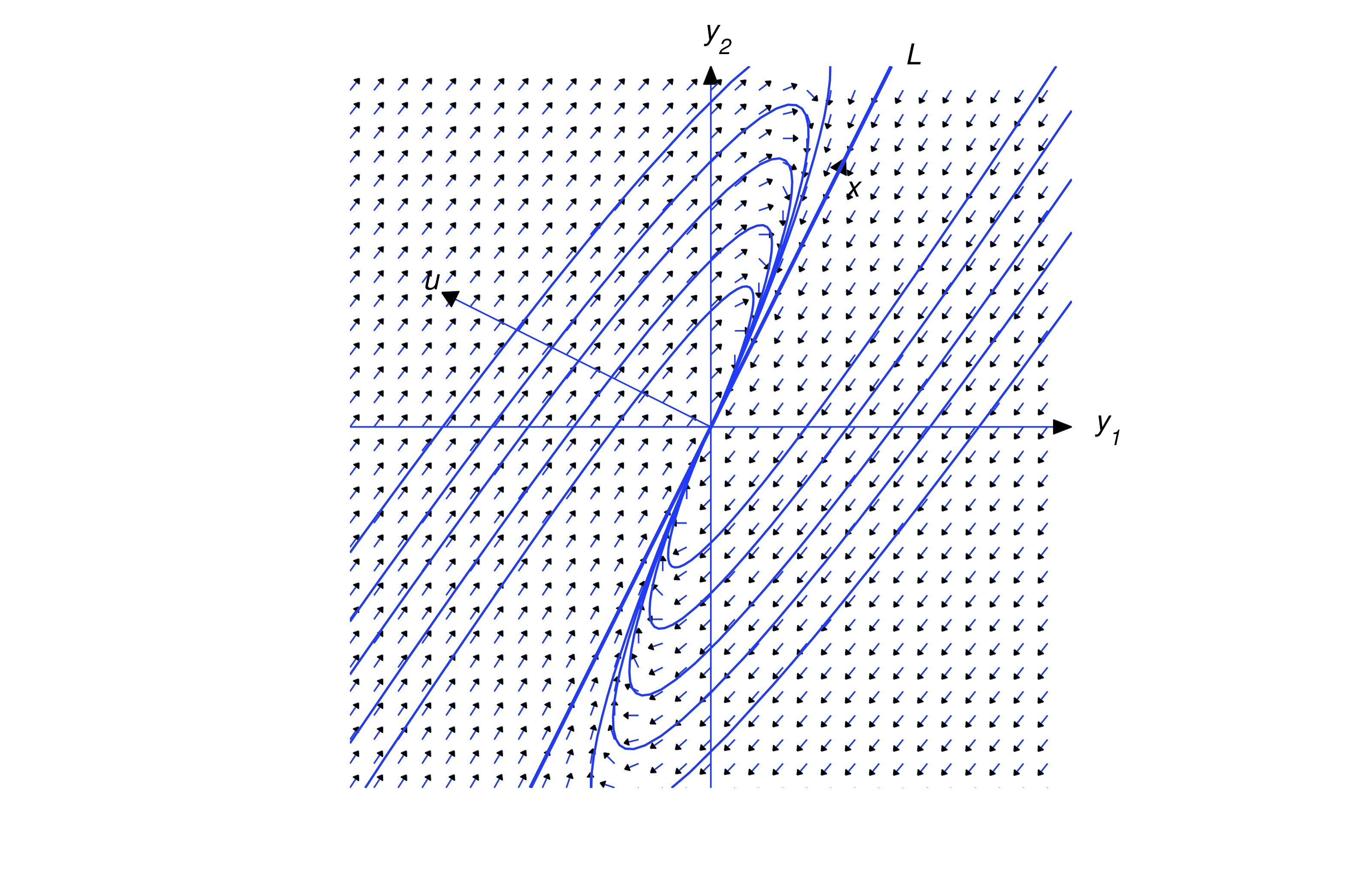
Let denote the line through the origin parallel to . By a half-line of we mean either of the rays obtained by removing the origin from . Eqn. (eq:10.5.20) is a parametric equation of the half-line of in the direction of if , or of the half-line of in the direction of if . The origin is the trajectory of the trivial solution .
Henceforth, we assume that . In this case, the trajectory of (eq:10.5.20) can’t intersect , since every point of is on a trajectory obtained by setting . Therefore the trajectory of (eq:10.5.20) must lie entirely in one of the open half-planes bounded by , but does not contain any point on . Since the initial point defined by is on the trajectory, we can determine which half-plane contains the trajectory from the sign of , as shown in the figure. For convenience we’ll call the half-plane where the positive half-plane. Similarly, the-half plane where is the negative half-plane. You should convince yourself that even though there are infinitely many vectors that satisfy (eq:10.5.21), they all define the same positive and negative half-planes. In the figures simply regard as an arrow pointing to the positive half-plane, since wen’t attempted to give its proper length or direction in comparison with . For our purposes here, only the relative orientation of and is important; that is, whether the positive half-plane is to the right of an observer facing the direction of , as in the figures below.
Or to the left of the observer, as shown below.
Multiplying (eq:10.5.20) by yields Since the last term on the right is dominant when is large, this provides the following information on the direction of :
- (a)
- Along trajectories in the positive half-plane (), the direction of approaches the direction of as and the direction of as .
- (b)
- Along trajectories in the negative half-plane (), the direction of approaches the direction of as and the direction of as .
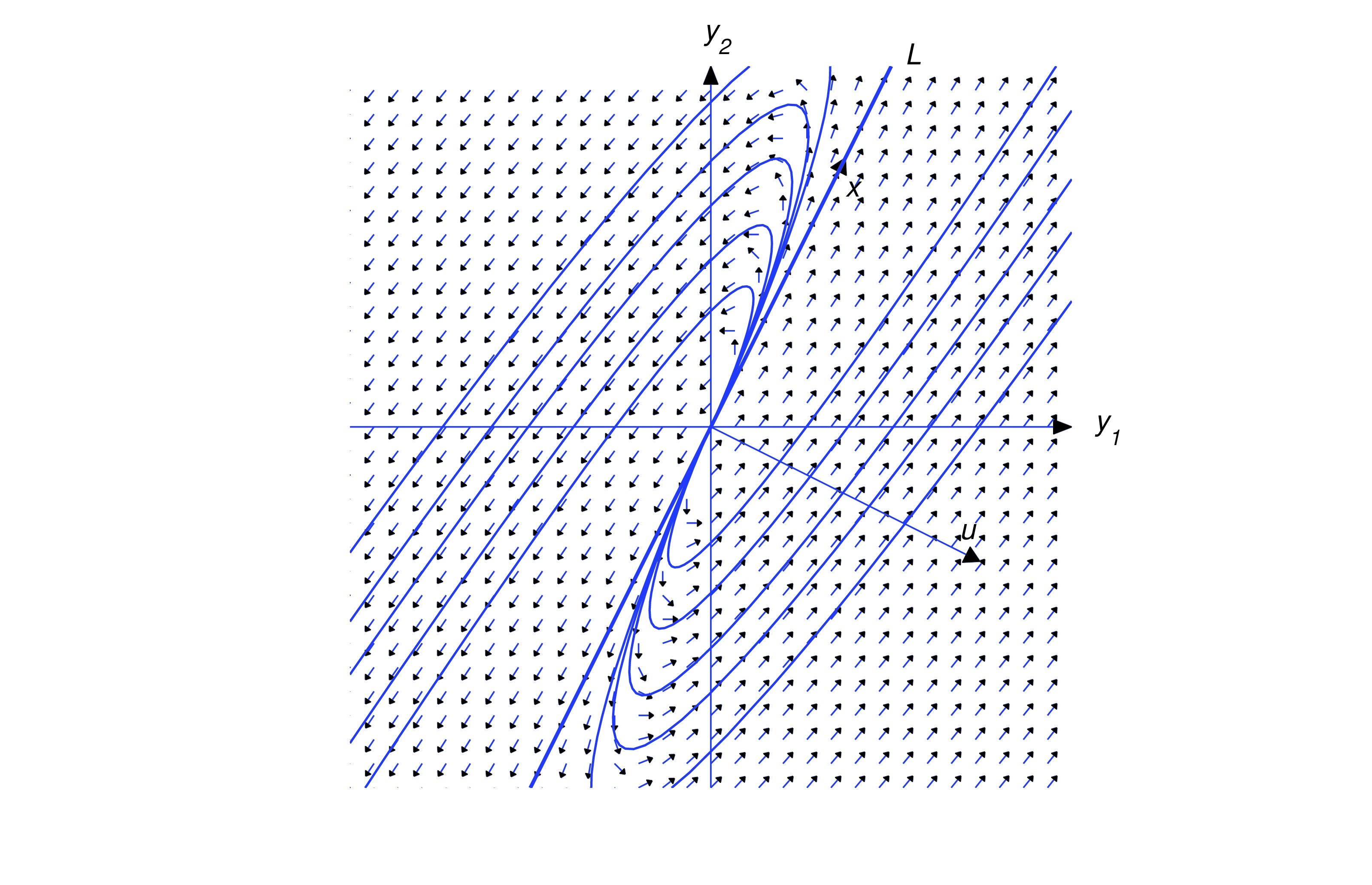
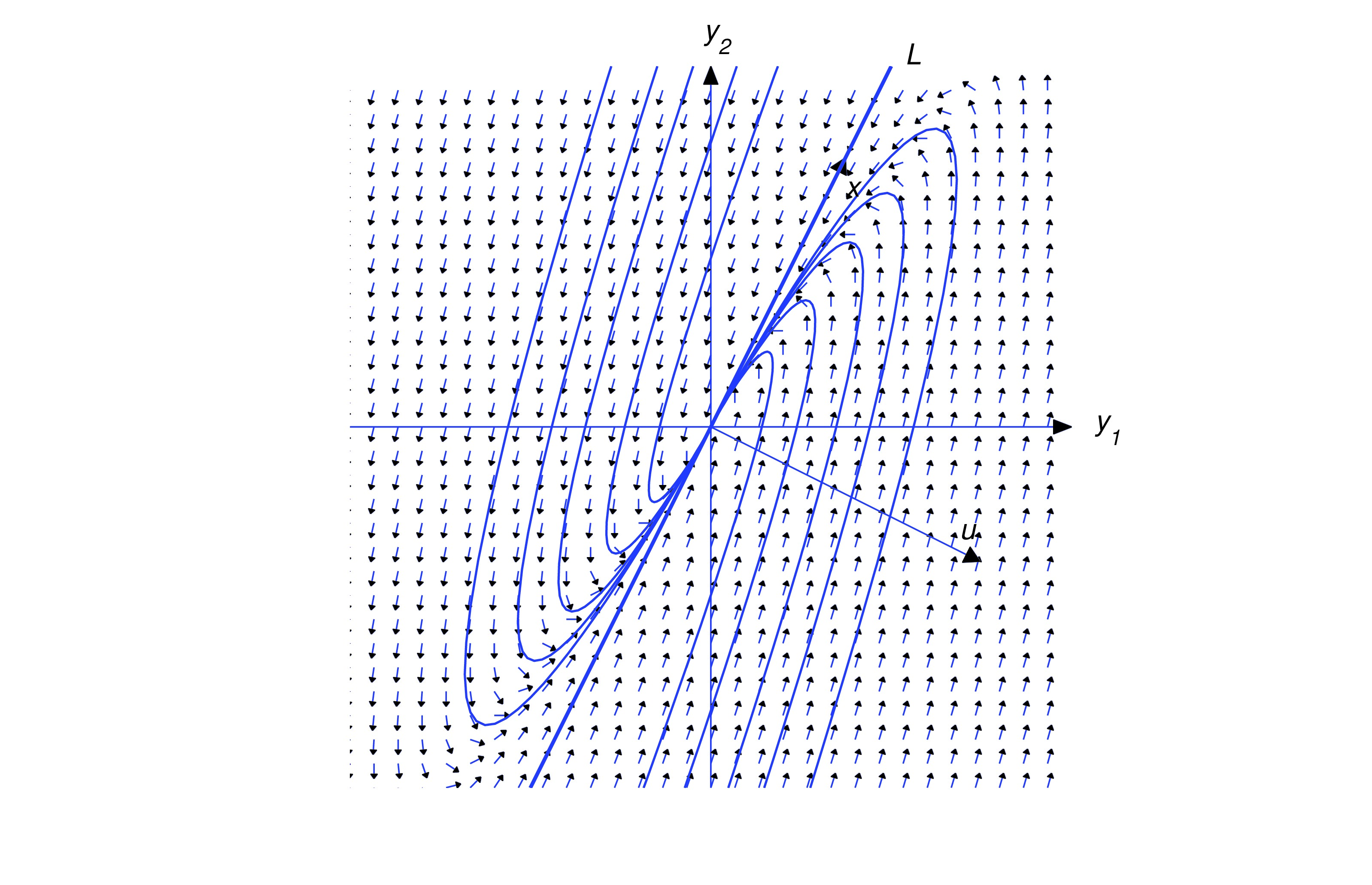
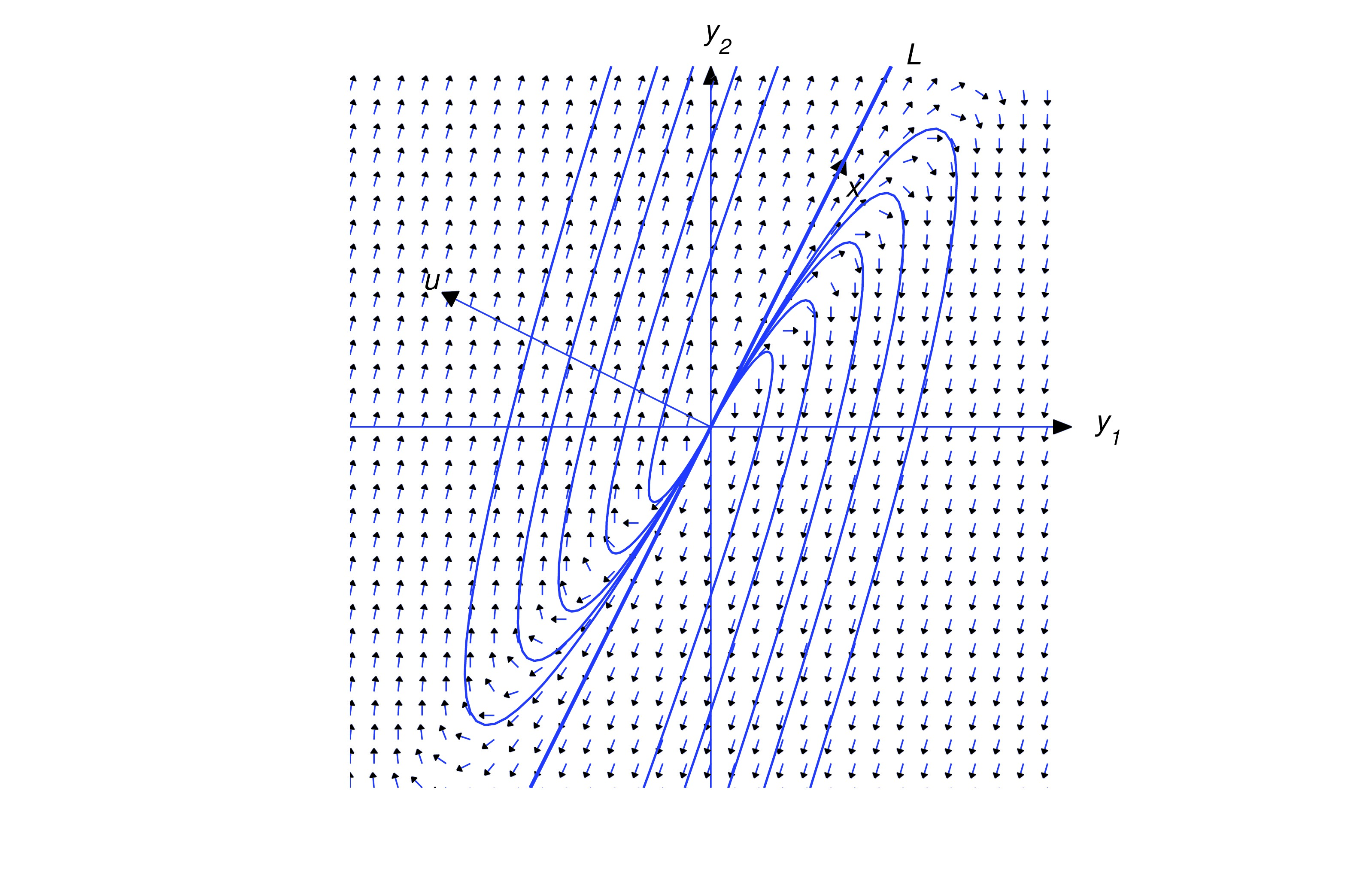
Since or there are four possible patterns for the trajectories of (eq:10.5.19), depending upon the signs of and .
The above figures illustrate these patterns, and reveal the following principle:
Text Source
Trench, William F., ”Elementary Differential Equations” (2013). Faculty Authored and Edited Books & CDs. 8. (CC-BY-NC-SA)