You are about to erase your work on this activity. Are you sure you want to do this?
Updated Version Available
There is an updated version of this activity. If you update to the most recent version of this activity, then your current progress on this activity will be erased. Regardless, your record of completion will remain. How would you like to proceed?
Mathematical Expression Editor
An experiment involving Newton’s Law of Cooling.
The purpose of this exercise is to deepen your understanding of Newton’s Law of
Heating (and Cooling) which is reviewed in Trench’s text in Section 4.2. A hands-on
activity will help to supplement and apply the background theory. Students will
record and predict the temperature of a potato baking in the oven and then
subsequently left out to cool. This experimental activity requires the use of an oven
thermometer, preferably a digital one that has a wire to allow readings with a closed
oven door. If you have or can borrow a thermometer, you can conduct this
experiment in your own kitchen. Particularly hungry students will opt to bake a few
potatoes and also be ready with some sour cream or blue cheese dressing.
Students without access to an oven may try the same experiment with the
potato submerged in boiling water. Overview in Section 4.2 of Trench’s text,
Newton’s Law of Cooling is summarized a first order differential equation:
This equation stipulates that , the time rate of change of the temperature of some
object, is linearly proportional to the difference between the temperature of that
object and the temperature of the medium or surroundings of the object . Trench
notes the ideal case where is perfectly constant, such as when an object is in a room
or a hot oven that remains at a constant temperature. A negative sign is placed
before the ”temperature decay constant” of the medium , which is itself some positive
number that will stipulate the relative rate of the object’s temperature change.
Observe that this differential equation has a very similar appearance to
one describing radioactive decay (or any natural decay problem). In fact,
heating or cooling of an object is essentially an exponential decay problem.
The quantity that decays in this case is the difference between the object
and its surroundings. This difference decays at a rate proportional to its
magnitude.
Predicting the heating process
Consider what Newton’s Law of Heating would predict for a potato heated in an
oven. Note that this law neglects some more complicated aspects of heating, so for
now you should only consider what the law itself would predict. Examine the
differential equation, and remember that k and Tm are constants. At what point
during the heating process will the rate of change of the temperature be the
largest? How will this rate change over time? Which of the following plots of
temperature vs. time most closely represents the behavior predicted by this
law?
Enter the ID number of the correct graph.
Expand for discussion.
Note that the final rate of change of the temperature is greater than the initial rate
of change. The temperature should asymptotically approach the temperature of the
medium because Newton’s Law of Heating shows that will get very small as
approaches . This plot suggests that the temperature of the object might
actually exceed the temperature of the surroundings, which is impossible.
Expand for discussion.
As the temperature of the object approaches that of the medium, the slope of the
tangent line approaches zero. Thus, this final attribute is correct. Note that Newton’s
Law of Heating predicts that the initial slope will be the greatest because the initial
difference between and is larger than after some heating has occurred. This law does
not predict any lag in the beginning of the heating process, although in reality some
lag may occur if the temperature of the inside of a larger object takes a bit longer to
begin heating up. This is one of the simplifications inherent in Newton’s Law of
Heating.
Expand for discussion.
The initial slope will be the greatest because the initial difference between and is
larger than after some heating has occurred. As the temperature of the object
approaches that of the medium, the slope approaches zero. Newton’s Law for Heating
thus predicts that the plot of temperature vs. time should be concave downward.
Take the derivative of both sides of the differential equation to see that is equal to .
Since the second derivative is a constant negative value, the curve is concave
downward.
Expand for discussion.
This graph does not capture how the rate of temperature change will – itself – vary
during the heating process. Note that the final rate of change of the temperature
should be small and the initial rate of change should be larger. The temperature
should asymptotically approach the temperature of the medium because
Newton’s Law of Heating shows that will become very small as T approaches .
Solving the differential equation
Recall that the differential equation bears a strong resemblance to an exponential
decay problem. As with that model, separation and integration provides a method to
quickly solve for temperature as a function of time:
Take a moment and attempt to solve this differential equation to find a solution for
temperature as a function of time. Don’t look ahead until you have found a solution
or are stuck. Look back to Trench’s use of ”separation of variables” in Examples 2.1.3
and 2.1.4 of his text.
The first step is to separate the equation, putting the dependent temperature
variable on the left hand side and the independent time () variable on the right
hand side. Integrating once produces a logarithm on the left side and an
explicit time variable on the right side, along with a constant of integration.
Next, we raise the natural base to the power of both sides, annihilating the
logarithm. The absolute value sign can be discarded by reversing the order of the
difference because — for heating — the surrounding temperature of the oven is
always greater than the temperature of the object (). This process produces
a new constant which must be positive. Applying an initial condition
allows the positive constant to be written in terms of the temperature of the
medium and the initial temperature of the object: The final solution gives
the temperature explicitly as a function of time and the other parameters.
With a given oven temperature and an initial temperature of the object only the
“temperature decay constant” of the medium needs to be specified to predict the
trajectory of temperature with time. Notice that at very long times the second term
decays to zero meaning that the object’s temperature will approach the temperature
of the surroundings.
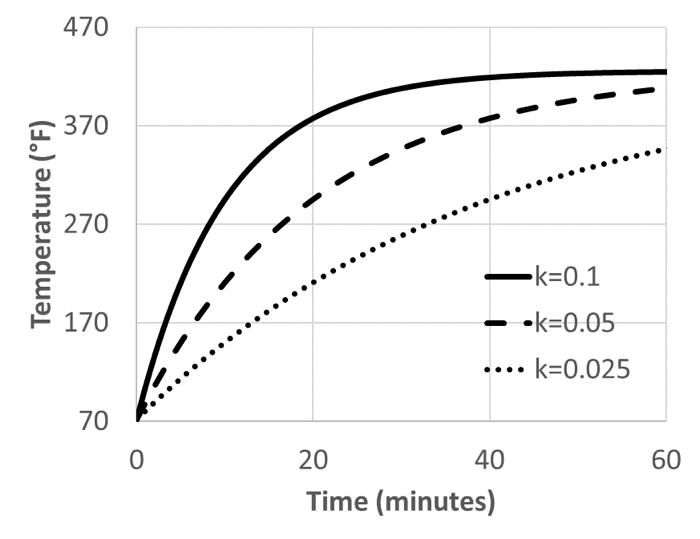
This solution is used to produce a plot of temperature vs. time for a potato heating
from room temperature towards an oven temperature of . Different sample
values of the temperature decay constant are used. Higher values of the
temperature decay constant correspond to faster heating towards the final
temperature.
Though we don’t yet have an estimate of for the potato and oven, we do have a
general idea of the shape and features of the heating curve. Before we proceed with
the experiment, we must discuss a complexity that has not yet been dealt with that
will limit the temperature of the potato while baking. This has to do with the
significant water content within the potato itself. Online sources suggest that it takes
almost an hour to bake potatoes at an oven temperature of but that it is ideal for
the potato to reach an internal temperature of . Recall that the boiling point of
water is , well below the oven temperature. This means that the temperature
of the potato will not exceed until all of the water vaporizes and leaves
the potato, which will not actually occur. This is fundamentally the same
phenomenon that one sees when boiling a pot of water at ambient pressure;
the water temperature will remain at the boiling point during the boiling
process. Uncooked potatoes are composed mainly of water and even baked
potatoes still have a significant water content. Therefore, these practical
limitations limit our potato’s temperature to about . We do not expect the
temperature of the potato to get anywhere near the temperature of the
oven.
The Hot Potato Experiment
In this experiment, we will record temperature data every minute during the first
twenty minutes of heating and then use that information to estimate the temperature
decay constant . This will allow us to make a prediction of the time necessary for the
potato to cool undisturbed until it is at a good eating temperature. Assemble the
following items in your kitchen while you preheat your oven to bake at :
A wired digital cooking thermometer to allow for real-time readings
without opening your oven door. In this example, an Oneida Model 31161
is used.
At least one medium or small baking potato such as a Russet variety.
The specific type of potato is likely unimportant but you should not cut
them or remove a significant quantity of the skin. It is advisable to poke
the potato with a fork or knife to allow water vapor to escape and avoid
breakage in the event that steam pressure builds up inside. The potato
should initially be at room temperature
Oven mitts, hot pads, or tongs for moving the potato in the hot oven.
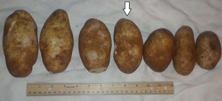
Here, a variety of potato sizes were baked at the same time, but only the
middle sized one marked with an arrow is monitored throughout the baking
process. The largest and smallest potatoes can be measured once later in the
process, but this is optional. (The largest and smallest potato were both
found to be very close to the temperature of the middle potato at the end of
baking.)
Caution: Avoid touching the hot potato, oven, or the thermometer wire.
Use oven mitts, hot pads, or tongs to avoid a burn.
Take the following steps to carry out this experiment:
(a)
Be sure that your temperature probe is functional with good batteries.
If left out in the open, it should read - steadily - somewhere near room
temperature (around ).
(b)
Insert the temperature probe into the center of the potato. If the potato
is at room temperature, the probe reading should stay roughly constant.
(c)
Before inserting the potato into the fully preheated oven, wait a couple
of minutes to make sure that the potato temperature is constant. While
you do that, prepare a notebook or computer spreadsheet to record the
temperature every minute for the first twenty minutes. Setting an alarm
to beep every one minute is a good way to remind you to write down the
temperature, but don’t lose track of the overall time. It is not a problem
if you miss an occasional reading.
(d)
Once the oven is fully preheated and the potato temperature is stabilized,
you are ready to begin. With oven mitts, hot pads, or tongs, insert the
potato into the oven and close the door over the probe wire. It is best to
keep the oven door closed during the entire course of the experiment so
that the oven temperature will remain as steady as possible.
(e)
Record the initial temperature as ”time zero” and for every minute
thereafter to at least twenty minutes. Tabulate and plot this data to use as
described below. You can probably do some of the analysis as the potato
finishes its hour in the oven and while it is left out to cool, though don’t
lose track of the time.
(f)
Continue heating the potato for a total of one hour, recording at least
the last few minutes of temperature in the oven. For illustration purposes,
most of the data over the hour-long heating process is included in this
example.
(g)
Remove the potato from the oven and set it on a plate or the stovetop
with the probe still inserted, recording the temperature every minute or
two until the potato cools to at least . This is the temperature at which
the average person would begin to be comfortable taking a bite. Use the
data you collected in the way described below to check your prediction of
the time necessary to cool. Below, the temperature during cooling of an
entire hour is included for illustration purposes.
The following data from the first twenty minutes of this example was collected and
plotted:
Your data and curve should be smooth but may only match this data approximately.
One noticeable feature of the plot is that the temperature increase lags at the
beginning because the center of the potato - where the probe is inserted - does not
immediately increase as fast as the outer portion of the potato. This effect means
that it will take longer for the potato to heat up than Newton’s Law of Heating
would predict. In order to estimate the “temperature decay constant”, we should
avoid using the data from the first several minutes of the experiment where the lag is
present. Using two data points after ten minutes offers an appropriate way to
make an estimate of . To do this, consider the original differential equation:
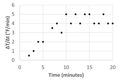
For smaller time steps, note that the change in temperature with time (the slope in
the plot above) does not change very much after the initial lag period:
After about ten minutes, is averaging around . Since this rate of change
in temperature is roughly constant, we may replace the derivative in the
differential equation with an average rate of change over some time step:
Rearranging the differential equation gives the following:
We could make an arbitrary selection of two data points at ten and fifteen minutes,
with associated temperatures of and . These times are far enough apart to
have a sizable temperature change where rounding to the nearest unit of
temperature will not impact the estimate. However, they are close enough
that the slope does not change much over that time range. Note that any
selection of two time-temperature data points after the initial ten minute lag
period would give a reasonable estimate. The change in temperature and time
may then be plugged into the above equation, and an average difference
of the medium minus object temperature () may be used since changes:
At ,
At ,
Average difference:
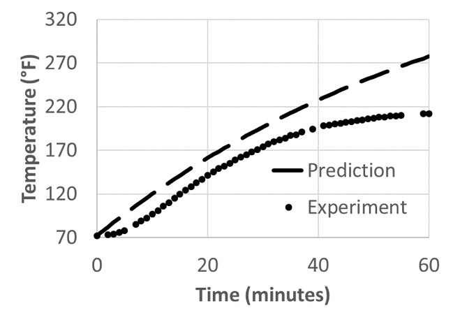
If this value of is used in the solution above, the prediction overestimates the
trajectory of the temperature after an hour of heating:
The first reason for this overestimation is the effect of the lag which is explained
above. As Newton’s Law of Heating does not predict this lag, the actual experimental
data remains well below the predicted temperature. The second reason for
overestimation is the effect of water vaporization. The potato’s temperature rises to
by the last couple minutes of the hour. By then the temperature has leveled off in an
asymptotic way, approaching the boiling point of water and falling well below the
predicted temperature. Just as with the temperature lag, Newton’s Law of Heating
has no way of predicting this complicated aspect of water vaporization. The
temperature of the potato would rise past this temperature only after all of the water
had evaporated, which would take a very long time and leave a very tough and
unappetizing spud. We can utilize the same value to estimate the time it will
take the potato to cool when left out on a plate or stovetop. At around , a
person could consider taking a bite without getting burned, so this will be our
target temperature. We will assume that the same basic relationships and
parameters for heating will apply with equal accuracy to the cooling process.
Newton’s Law applies equally to heating and cooling, so we can use the
same differential equation and solution. The only difference here is that
the medium temperature is room temperature, which is in this example.
Now, , the initial temperature, is the temperature out of the oven. Zero
time is considered to be when the potato is removed from the oven. In this
example, that is . Your potato will likely be at or near this temperature
when it finishes its hour in the oven. Using the numbers particular to your
experiment, plug everything into the solution and solve for , which is the time
(in minutes) that the potato will take to reach a target temperature of .
Using the numbers in this example, the necessary cooling time is found to be about
minutes. Note that the potato would cool much faster if you cut or mashed it.
Increasing the surface area promotes faster cooling. Yet cutting or mashing would
significantly increase the temperature decay constant and our previous value would
not apply.
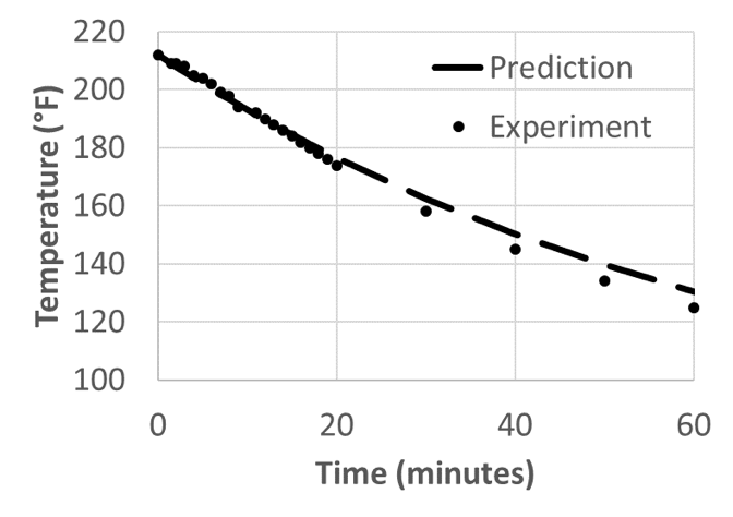
In this experiment, the potato cools to the target temperature of after about
minutes, which means our prediction had a high degree of accuracy as it was within
one minute of the observed time. The following figure shows a very good correlation
between the prediction and the experimental cooling data over an entire
hour:
How close was your prediction? Do you see a lag with the cooling process as well? A
small lag is noticeable in the figure above, with the potato temperature staying
slightly warmer than predicted in the first several minutes. It is remarkable that an
uncut potato can stay warm for so long. In days past, those who lived in cold
climates would use hot potatoes as hand warmers (and then lunch!). One such use of
hot potatoes in coat pockets is mentioned in the novel Little House in the Big Woods
by Laura Ingalls Wilder.