Need Abstract
Euler’s Method
Introduction
In science and mathematics, finding exact solutions to differential equations is not always possible. We have already seen that slope fields give us a powerful way to understand the qualitative features of solutions. Sometimes we need a more precise quantitative understanding, meaning we would like numerical approximations of the solutions.
If an initial value problem
can’t be solved analytically, it’s necessary to resort to numerical methods to obtain useful approximations to a solution.The simplest numerical method for solving (eq:3.1.1) is Euler’s method. This method is so crude that it is seldom used in practice; however, its simplicity makes it useful for illustrative purposes.
Euler’s method is based on the assumption that the tangent line to the integral curve of (eq:3.1.1) at approximates the integral curve over the interval . Since the slope of the integral curve of (eq:3.1.1) at is , the equation of the tangent line to the integral curve at is
Setting in (eq:3.1.2) yields
as an approximation to . Since is known, we can use (eq:3.1.3) with to compute However, setting in (eq:3.1.3) yields which isn’t useful, since we don’t know . Therefore we replace by its approximate value and redefine Having computed , we can compute In general, Euler’s method starts with the known value and computes successively using the formulaThe next example illustrates the computational procedure indicated in Euler’s method.
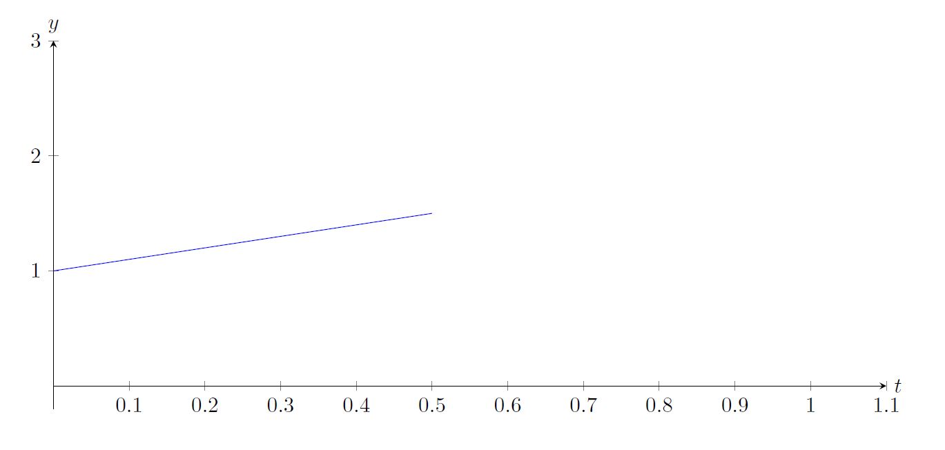
Consider the following differential equation
Let us approximate the solution using just two subintervals Since , we know that by (eq:3.1.3).
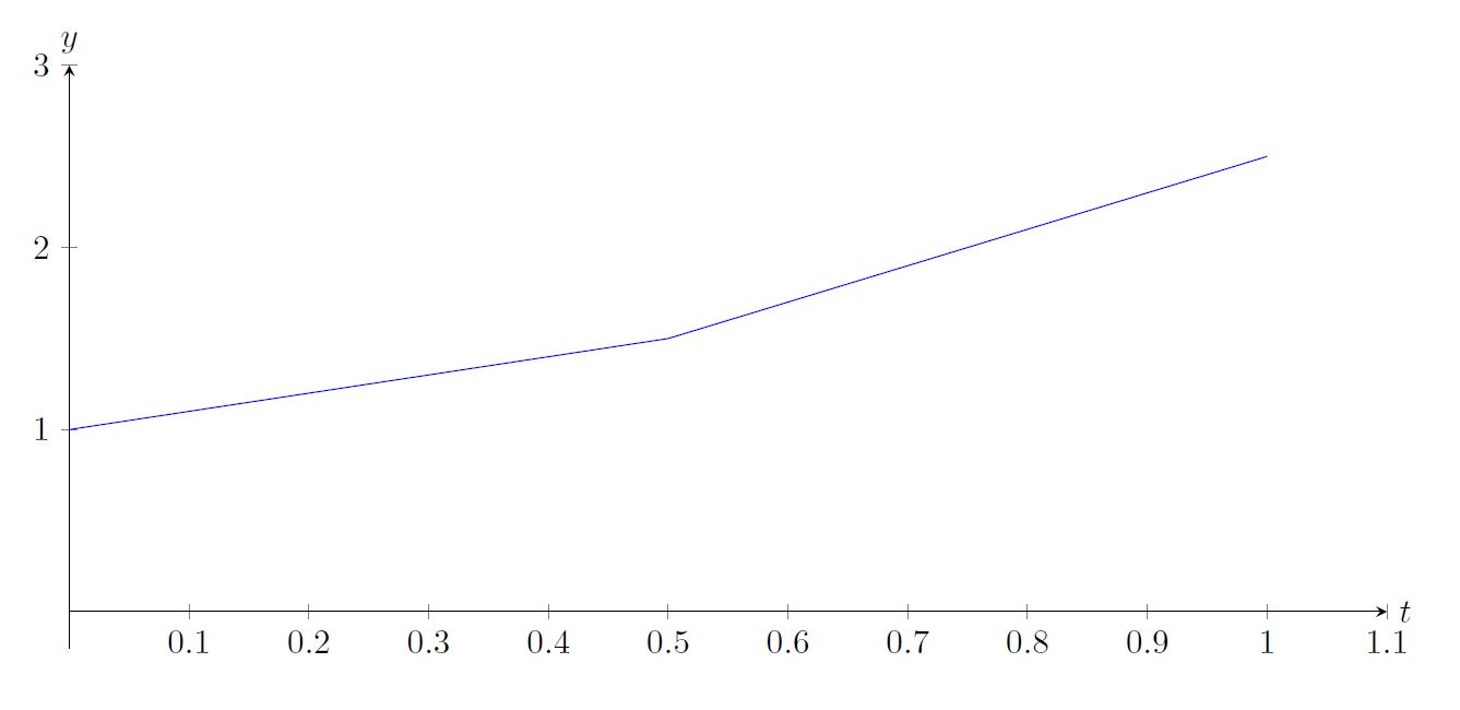
But now, we have so
Plotting our approximation with the actual solution we find:
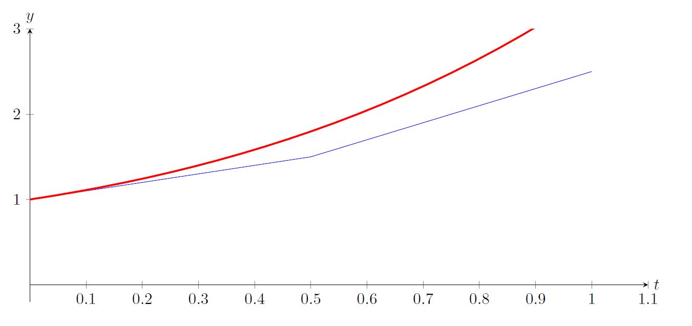
This approximation could be improved by using more subintervals. Use the Sage Cell below to increase the number of subintervals to improve the approximation.
The Sage Cell below illustrates Example ex:eulerIntro2 graphically. You can adjust the number of subintervals to see how the approximation is affected. You can also change the the interval, just for fun.
Sources of Error
When using numerical methods we’re interested in computing approximate values of the solution of (eq:3.1.1) at equally spaced points in an interval . Thus, where We’ll denote the approximate values of the solution at these points by ; thus, is an approximation to . We’ll call the error at the th step. Because of the initial condition , we’ll always have . However, in general if .
We encounter two sources of error in applying a numerical method to solve an initial value problem:
- The formulas defining the method are based on some sort of approximation. Errors due to the inaccuracy of the approximation are called truncation errors.
- Computers do arithmetic with a fixed number of digits, and therefore make errors in evaluating the formulas defining the numerical methods. Errors due to the computer’s inability to do exact arithmetic are called roundoff errors.
Since a careful analysis of roundoff error is beyond the scope of this book, we’ll consider only truncation errors.
You can see that decreasing the step size improves the accuracy of Euler’s method. For example, Based on this scanty evidence, you might guess that the error in approximating the exact solution at a fixed value of by Euler’s method is roughly halved when the step size is halved. You can find more evidence to support this conjecture by examining the table below which lists the approximate values of at .
Use the Sage Cell below to explore the error in Example example:3.1.2 visually by changing the size () of the subintervals.
Since we think it’s important in evaluating the accuracy of the numerical methods that we’ll be studying in this chapter, we often include a column listing values of the exact solution of the initial value problem, even if the directions in the example or exercise don’t specifically call for it. If quotation marks are included in the heading, the values were obtained by applying the Runge-Kutta method in a way that’s explained in Section 3.3. If quotation marks are not included, the values were obtained from a known formula for the solution. In either case, the values are exact to eight places to the right of the decimal point.
Truncation Error in Euler’s Method
Consistent with the results indicated in Tables table:3.1.1–table:3.1.4, we’ll now show that under reasonable assumptions on there’s a constant such that the error in approximating the solution of the initial value problem at a given point by Euler’s method with step size satisfies the inequality where is a constant independent of .
There are two sources of error (not counting roundoff) in Euler’s method:
- (a)
- The error committed in approximating the integral curve by the tangent line (eq:3.1.2) over the interval .
- (b)
- The error committed in replacing by in (eq:3.1.2) and using (eq:3.1.4) rather than (eq:3.1.2) to compute .
Euler’s method assumes that defined in (eq:3.1.2) is an approximation to . We call the error in this approximation the local truncation error at the th step, and denote it by ; thus,
We’ll now use Taylor’s theorem to estimate , assuming for simplicity that , , and are continuous and bounded for all . Then exists and is bounded on . To see this, we differentiate to obtainNote that the magnitude of the local truncation error in Euler’s method is determined by the second derivative of the solution of the initial value problem. Therefore the local truncation error will be larger where is large, or smaller where is small.
Since the local truncation error for Euler’s method is , it’s reasonable to expect that halving reduces the local truncation error by a factor of . This is true, but halving the step size also requires twice as many steps to approximate the solution at a given point. To analyze the overall effect of truncation error in Euler’s method, it’s useful to derive an equation relating the errors To this end, recall that
and Subtracting (eq:3.1.12) from (eq:3.1.11) yields The last term on the right is the local truncation error at the th step. The other terms reflect the way errors made at previous steps affect . Since , we see from (eq:3.1.13) that Since we assumed that is continuous and bounded, the mean value theorem implies that where is between and . Therefore for some constant . From this and (eq:3.1.14), For convenience, let . Since , applying (eq:3.1.15) repeatedly yieldsRecalling the formula for the sum of a geometric series, we see that (since ). From this and (eq:3.1.16),
Since Taylor’s theorem implies that (verify), This and (eq:3.1.17) imply that with Because of (eq:3.1.18) we say that the global truncation error of Euler’s method is of order , which we write as .Semilinear Equations and Variation of Parameters
An equation that can be written in the form
with is said to be semilinear. (Of course, (eq:3.1.19) is linear if is independent of .) One way to apply Euler’s method to an initial value problem for (eq:3.1.19) is to think of it as where However, we can also start by applying variation of parameters to (eq:3.1.20), as in Sections 2.1 and 2.4; thus, we write the solution of (eq:3.1.20) as , where is a nontrivial solution of the complementary equation . Then is a solution of (eq:3.1.20) if and only if is a solution of the initial value problem We can apply Euler’s method to obtain approximate values of this initial value problem, and then take as approximate values of the solution of (eq:3.1.20). We’ll call this procedure the Euler semilinear method.The next two examples show that the Euler and Euler semilinear methods may yield drastically different results.
It’s easy to see why Euler’s method yields such poor results. Recall that the constant in (eq:3.1.10) – which plays an important role in determining the local truncation error in Euler’s method – must be an upper bound for the values of the second derivative of the solution of the initial value problem (eq:3.1.22) on . The problem is that assumes very large values on this interval. To see this, we differentiate (eq:3.1.24) to obtain where the second equality follows again from (eq:3.1.24). Since (eq:3.1.23) implies that if , For example, letting shows that .
item:3.1.4b Since is a solution of the complementary equation , we can apply the Euler semilinear method to (eq:3.1.22), with The results listed in the following table are clearly better than those obtained by Euler’s method.
We can’t give a general procedure for determining in advance whether Euler’s method or the semilinear Euler method will produce better results for a given semilinear initial value problem (eq:3.1.19). As a rule of thumb, the Euler semilinear method will yield better results than Euler’s method if is small on , while Euler’s method yields better results if is large on . In many cases the results obtained by the two methods don’t differ appreciably. However, we propose the an intuitive way to decide which is the better method: Try both methods with multiple step sizes, as we did in Example example:3.1.4, and accept the results obtained by the method for which the approximations change less as the step size decreases.
Applying the Euler semilinear method with yields the results in the table below.
Since the latter are clearly less dependent on step size than the former, we conclude that the Euler semilinear method is better than Euler’s method for (eq:3.1.25). This conclusion is supported by comparing the approximate results obtained by the two methods with the “exact” values of the solution.
Applying the Euler semilinear method with yields the following.
Noting the close agreement among the three columns of the first table (at least for larger values of ) and the lack of any such agreement among the columns of the second table, we conclude that Euler’s method is better than the Euler semilinear method for (eq:3.1.26). Comparing the results with the exact values supports this conclusion.
In the next two modules we’ll study other numerical methods for solving initial value problems, called the improved Euler method, the midpoint method, Heun’s method and the Runge-Kutta method. If the initial value problem is semilinear as in (eq:3.1.19), we also have the option of using variation of parameters and then applying the given numerical method to the initial value problem (eq:3.1.21) for . By analogy with the terminology used here, we’ll call the resulting procedure the improved Euler semilinear method, the midpoint semilinear method, Heun’s semilinear method or the Runge-Kutta semilinear method, as the case may be.
Text Source
MOOCulus, Numerical Methods (CC-BY-NC-SA)
Trench, William F., ”Elementary Differential Equations” (2013). Faculty Authored and Edited Books & CDs. 8. (CC-BY-NC-SA)