Uncoupled Linear Systems of Two Equations

$\newenvironment {prompt}{}{} \newcommand {\Sec }[2]{\section {#1}} \newcommand {\trademark }[0]{{R\!\!\!\!\!\bigcirc }} \newcommand {\EXER }[0]{\section *{Exercises}} \newcommand {\CEXER }[0]{} \newcommand {\TEXER }[0]{} \newcommand {\R }[0]{\mbox {$\Bbb {R}$}} \newcommand {\C }[0]{\mbox {$\Bbb {C}$}} \newcommand {\Z }[0]{\mbox {$\Bbb {Z}$}} \newcommand {\N }[0]{\mbox {$\Bbb {N}$}} \newcommand {\D }[0]{\mbox {{\bf D}}} \newcommand {\setmin }[0]{\;\mbox {--}\;} \newcommand {\Matlab }[0]{{M\small {AT\-LAB}} } \newcommand {\Matlabp }[0]{{M\small {AT\-LAB}}} \newcommand {\computer }[0]{\Matlab Instructions} \newcommand {\half }[0]{\mbox {$\frac {1}{2}$}} \newcommand {\compose }[0]{\raisebox {.15ex}{\mbox {{\scriptsize $\circ $}}}} \newcommand {\AND }[0]{\quad \mbox {and}\quad } \newcommand {\vect }[2]{\left (\begin {array}{c} #1_1 \\ \vdots \\ #1_{#2}\end {array}\right )} \newcommand {\mattwo }[4]{\left (\begin {array}{rr} #1 & #2\\ #3 &#4\end {array}\right )} \newcommand {\mattwoc }[4]{\left (\begin {array}{cc} #1 & #2\\ #3 &#4\end {array}\right )} \newcommand {\vectwo }[2]{\left (\begin {array}{r} #1 \\ #2\end {array}\right )} \newcommand {\vectwoc }[2]{\left (\begin {array}{c} #1 \\ #2\end {array}\right )} \newcommand {\inv }[0]{^{-1}} \newcommand {\CC }[0]{{\cal C}} \newcommand {\CCone }[0]{\CC ^1} \newcommand {\Span }[0]{{\rm span}} \newcommand {\rank }[0]{{\rm rank}} \newcommand {\trace }[0]{{\rm tr}} \newcommand {\RE }[0]{{\rm Re}} \newcommand {\IM }[0]{{\rm Im}} \newcommand {\nulls }[0]{{\rm null\;space}} \newcommand {\dps }[0]{\displaystyle } \newcommand {\arraystart }[0]{\renewcommand {\arraystretch }{1.8}} \newcommand {\arrayfinish }[0]{\renewcommand {\arraystretch }{1.2}} \newcommand {\Start }[1]{\vspace {0.08in}\noindent {\bf Section~\ref {#1}}} \newcommand {\exer }[1]{\noindent {\bf \ref {#1}}} \newcommand {\ans }[0]{} \newcommand {\matthree }[9]{\left (\begin {array}{rrr} #1 & #2 & #3 \\ #4 & #5 & #6 \\ #7 & #8 & #9\end {array}\right )} \newcommand {\cvectwo }[2]{\left (\begin {array}{c} #1 \\ #2\end {array}\right )} \newcommand {\cmatthree }[9]{\left (\begin {array}{ccc} #1 & #2 & #3 \\ #4 & #5 & #6 \\ #7 & #8 & #9\end {array}\right )} \newcommand {\vecthree }[3]{\left (\begin {array}{r} #1 \\ #2 \\ #3\end {array}\right )} \newcommand {\cvecthree }[3]{\left (\begin {array}{c} #1 \\ #2 \\ #3\end {array}\right )} \newcommand {\cmattwo }[4]{\left (\begin {array}{cc} #1 & #2\\ #3 &#4\end {array}\right )} \newcommand {\thehelp }[0]{\thesection .\arabic {equation}} \newcommand {\matlabEquation }[0]{\let \oldtheequation \theequation \renewcommand {\theequation }{\oldtheequation *}\begin {equation}} \newcommand {\HyperFirstAtBeginDocument }[0]{\AtBeginDocument } \newcommand {\epstopdfsetup }[0]{\setkeys {ETE}} changed the theorem header of amsthm failed\MessageBreak }}} \newcommand {\GetTitleStringSetup }[0]{\setkeys {gettitlestring}} \newcommand {\Sectionformat }[2]{#1} \newcommand {\arraystretch }[0]{1.8} \newcommand {\arraystretch }[0]{1.8} \newcommand {\arraystretch }[0]{1.0} \newcommand {\arraystretch }[0]{1.8} \newcommand {\arraystretch }[0]{1.0}$ $% This file was *autogenerated* from uncoupledLinearSystemsOfTwoEquations.sagetex.sage with % sagetex.py version 2015/08/26 v3.0-92d9f7a %81acde9d6812ecfdfea7aa67ed0cc0b1% md5sum of corresponding .sage file (minus "goboom","current_tex_line",and pause/unpause lines)$

An autonomous system of two (first order) differential equations has the form

$\begin{equation} \label{e:aut2} \begin{array}{lll} \dps \frac{dx}{dt}(t) & = & f(x(t),y(t)) \\ \dps \frac{dy}{dt}(t) & = & g(x(t),y(t)), \end{array} \end{equation}$ where $f$ and $g$ are functions of the two variables $x$ and $y$ . Solutions to (??) are pairs of functions $(x(t),y(t))$ .

As in the single equation (??), the simplest solutions are equilibria. An equilibrium solution to (??) is a solution where both functions $x(t)$ and $y(t)$ are constant functions; that is, $x(t) = x_0 \AND y(t)=y_0.$ For equilibria, it follows that both $\frac {dx}{dt} = 0 \AND \frac {dy}{dt} = 0.$ Hence, equilibria of (??) can be found by simultaneously solving the equations

$\begin{eqnarray*} f(x,y) & = & 0 \\ g(x,y) & = & 0. \end{eqnarray*}$

An autonomous linear system of ordinary differential equations has the form

$\begin{equation} \label{e:autlin} \begin{array}{lll} \dps \frac{dx}{dt}(t) & = & a x(t) + b y(t) \\ \dps \frac{dy}{dt}(t) & = & c x(t) + d y(t), \end{array} \end{equation}$ where $a,b,c,d$ are real constants. Note that the origin $(x(t),y(t))=(0,0)$ is always an equilibrium for a linear system.

We begin our discussion of linear systems of ordinary differential equations by considering uncoupled systems of the form

$\begin{equation} \label{lin2} \begin{array}{lll} \dps \frac{dx}{dt}(t) & = & a x(t) \\ \dps \frac{dy}{dt}(t) & = & d y(t). \end{array} \end{equation}$ Since the system is uncoupled (that is, the equation for $\dot {x}$ does not depend on $y$ and the equation for $\dot {y}$ does not depend on $x$ ), we can solve this system by solving each equation independently, as we did for (??): $\begin{equation} \label{e:explicitsoln} \begin{array}{ccc} x(t) & = & x_0e^{at} \\ y(t) & = & y_0e^{dt}. \end{array} \end{equation}$ There are now two initial conditions that are identified by $x(0) = x_0 \AND y(0) = y_0.$

Having found all the solutions to (??) in (??), we now explore the geometry of the phase plane for these uncoupled systems both analytically and by using MATLAB.

Asymptotic Stability of the Origin

As we did for the single equation (??), we ask what happens to solutions to (??) starting at $(x_0,y_0)$ as time $t$ increases. That is, we compute $\lim _{t\to \infty }(x(t),y(t))=\lim _{t\to \infty }(x_0e^{a t},y_0e^{d t}).$ This limit is $(0,0)$ when both $a<0$ and $d<0$ ; but if either $a$ or $d$ is positive, then most solutions diverge to infinity, since either $\lim _{t\to \infty }|x(t)| =\infty \quad \mbox { or } \quad \lim _{t\to \infty }|y(t)| =\infty .$

Roughly speaking, an equilibrium $(x_0,y_0)$ is asymptotically stable if every trajectory $(x(t),y(t))$ beginning from an initial condition near $(x_0,y_0)$ stays near $(x_0,y_0)$ for all positive $t$ , and $\lim _{t\to \infty }(x(t),y(t)) = (x_0,y_0).$ The equilibrium is unstable if there are trajectories with initial conditions arbitrarily close to the equilibrium that move far away from that equilibrium.

At this stage, it is not clear how to determine whether the origin is asymptotically stable for a general linear system (??). However, for uncoupled linear systems we have shown that the origin is an asymptotically stable equilibrium when both $a < 0$ and $d < 0$ . If either $a >0$ or $d > 0$ , then $(0,0)$ is unstable.

Invariance of the Axes

There is another observation that we can make for uncoupled systems. Suppose that the initial condition for an uncoupled system lies on the $x$ -axis; that is, suppose $y_0=0$ . Then the solution $(x(t),y(t))=(x_0e^{at},0)$ also lies on the $x$ -axis for all time. Similarly, if the initial condition lies on the $y$ -axis, then the solution $(0,y_0e^{dt})$ lies on the $y$ -axis for all time.

This invariance of the coordinate axes for uncoupled systems follows directly from (??). It turns out that many linear systems of differential equations have invariant lines; this is a topic to which we return later in this chapter.

Generating Phase Space Pictures with pplane5

How can we visualize a solution $(x(t),y(t))$ to a system of differential equations (??)? The time series approach suggests that we should graph $(x(t),y(t))$ as a function of $t$ ; that is, we should plot the curve $(t,x(t),y(t))$ in three dimensions. Using MATLAB it is possible to plot such a graph — but such a graph by itself is difficult to interpret. Alternatively, we could graph either of the functions $x(t)$ or $y(t)$ by themselves as we do for solutions to single equations — but then some information is lost.

The method we prefer is the phase space plot obtained by thinking of $(x(t),y(t))$ as the position of a particle in the $xy$ -plane at time $t$ . We then graph the point $(x(t),y(t))$ in the plane as $t$ varies. When looking at phase space plots, it is natural to call solutions trajectories, since we can imagine that we are watching a particle moving in the plane as time changes.

We begin by considering uncoupled linear equations. As we saw, when the initial conditions are on the coordinate axes (either $(x_0,0)$ or $(0,y_0)$ ), the solutions remain on the coordinate axes. For these initial conditions, the equations behave as if they were one dimensional. However, if we consider an initial condition $(x_0,y_0)$ that is not on a coordinate axis, then even for an uncoupled system it is a little difficult to see what the trajectory looks like. At this point it is useful to use the computer.

The method used to integrate planar systems of autonomous differential equations is similar to that used to integrate nonautonomous single equations in dfield5. The solution curve $(x(t),y(t))$ to (??) at a point $(x_0,y_0)$ is tangent to the direction $(f(x_0,y_0),g(x_0,y_0))$ . So the differential equation solver plots the direction field $(f,g)$ and then finds curves that are tangent to these vectors at each point in time.

The program pplane5, written by John Polking, is the two-dimensional analog of pline. In MATLAB type

pplane5

and the window with the PPLANE5 Setup appears. pplane5 has a number of preprogrammed differential equations listed in a menu accessed by clicking on Gallery. To explore linear systems, choose linear system in the Gallery. (Note that the parameters in the linear system are given by capitals rather than lower case a,b,c,d.)

To integrate the uncoupled linear system, set the parameters $b$ and $c$ equal to zero. We now have the system (??) with $a = 2$ and $d = -3$ . After pushing Proceed, a display window similar to dfield5 appears. The main difference is that the plane is filled by vectors $(f,g)$ indicating directions, rather than by line segments indicating slopes.

As with dfield5 we may start the computations by clicking with a mouse button on an initial value $(x_0,y_0)$ . For example, if we click approximately onto $(x(0),y(0))=(x_0,y_0)=(1,1)$ , then the trajectory in the upper right quadrant of Figure ?? displays.

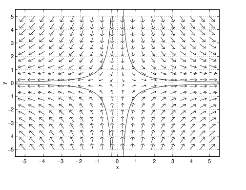
Figure 1: PPLANE5 Display for (??) with $a=2$ , $d=-3$ and $x,y\in [-5,5]$ . Solutions going through $(\pm 1,\pm 1)$ are shown.

First pplane5 draws the trajectory in forward time for $t\ge 0$ and then it draws the trajectory in backwards time for $t\le 0$ . More precisely, when we click on a point $(x_0,y_0)$ in the $(x,y)$ -plane, pplane5 computes that part of the solution that lies inside the specified display window and that goes through this point. For linear systems there is precisely one solution that goes through a specified point in the $(x,y)$ -plane. We prove this fact in Section ??.

Saddles, Sinks, and Sources for the Uncoupled System (??)

In a qualitative fashion, the trajectories of uncoupled linear systems are determined by the invariance of the coordinate axes and by the signs of the constants $a$ and $d$ .

Saddles: $ad<0$

In Figure ??, where $a=2>0$ and $d=-3<0$ , the origin is a saddle. If we choose several initial values $(x_0,y_0)$ one after another, then we find that as time increases all solutions approach the $x$ -axis. That is, if $(x(t),y(t))$ is a solution to this system of differential equations, then $\lim _{t\to \infty }y(t)=0$ . This observation is particularly noticeable when we choose initial conditions close to the origin $(0,0)$ . On the other hand, solutions also approach the $y$ -axis as $t\to -\infty$ . These qualitative features of the phase plane are valid whenever $a>0$ and $d<0$ .

When $a<0$ and $d>0$ , then the origin is also a saddle — but the roles of the $x$ and $y$ axes are reversed.

Sinks: $a<0$ and $d<0$

Now change the parameter $a$ to $-1$ . After clicking on Proceed and specifying several initial conditions, we see that all solutions approach the origin as time tends to infinity. Hence — as mentioned previously, and in contrast to saddles — the equilibrium $(0,0)$ is asymptotically stable. Observe that solutions approach the origin on trajectories that are tangent to the $x$ -axis. Since $d<a<0$ , the trajectory decreases to zero faster in the $y$ direction than it does in the $x$ -direction. If you change parameters so that $a<d<0$ , then trajectories will approach the origin tangent to the $y$ -axis.

Sources: $a>0$ and $d>0$

Choose the constants $a$ and $d$ so that both are positive. In forward time, all trajectories, except the equilibrium at the origin, move towards infinity and the origin is called a source.

Time Series Using pplane5

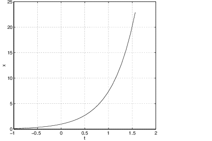
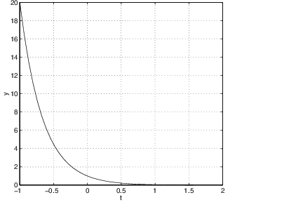
We may also use pplane5 to graph the time series of the single components $x(t)$ and $y(t)$ of a solution $(x(t),y(t))$ . For this we choose x vs. t from the Graph menu. After using the mouse to select a solution curve, another window with the title PPLANE5 t-plot appears. There the time series of $x(t)$ is shown. For example, when the differential equation is a sink, we observe that this component approaches $0$ as time $t$ tends to infinity. We may also display the time series of both components $x(t)$ and $y(t)$ simultaneously by clicking on Both in the PPLANE5 t-plot window. Again we see that both $x(t)$ and $y(t)$ tend to $0$ for increasing $t$ .

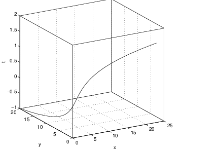
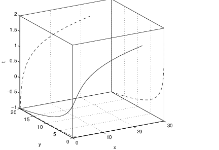
We may also visualize the time series of $x(t)$ and $y(t)$ in the three-dimensional $(x,y,t)$ -space. To see this, click onto 3 D and a curve $(x(t),y(t),t)$ becomes visible. Since $x(t)$ and $y(t)$ approach $0$ for $t\to \infty$ we see that this curve approaches the $t$ -axis for increasing time $t$ . Finally, we may look at all the different visualizations — the phase space plot, the time series for $x(t)$ and $y(t)$ and the three-dimensional representation of the solution — by clicking the Composite button. See Figure ??.

Figure 2: PPLANE5 Display for (??) with $a=2$ , $d=-3$ and $x\in [0,25], y\in [0,20]$ . The solution going through $(1,1)$ is shown. UL: $(t,x(t))$ ; UR: $(t,y(t))$ ; LL: $(x(t),y(t),t)$ ; LR: all plots.

Exercises

In Exercises ?? – ?? find all equilibria of the given system of nonlinear autonomous differential equations.

$\begin{eqnarray*} \dot{x} & = & x - y\\ \dot{y} & = & x^2 - y. \end{eqnarray*}$

$\begin{eqnarray*} \dot{x} & = & x^2 - xy\\ \dot{y} & = & x^2 + y^2 - 4. \end{eqnarray*}$

In Exercises ?? – ?? consider the uncoupled system of differential equations (??). For each choice of $a$ and $d$ , determine whether the origin is a saddle, source, or sink.

$a=1$ and $d=-1$ .

$a=-0.01$ and $d=-2.4$ .

$a=0$ and $d=-2.3$ .

Let $(x(t),y(t))$ be the solution (??) of (??) with initial condition $(x(0),y(0))=(x_0,y_0)$ , where $x_0\neq 0 \neq y_0$ .

Show that the points $(x(t),y(t))$ lie on the curve whose equation is: $y_0^ax^d - x_0^dy^a = 0.$
Verify that if $a=1$ and $d=2$ , then the solution lies on a parabola tangent to the $x$ -axis.

Use the phase plane picture given in Figure ?? to draw the time series $x(t)$ when $(x(0),y(0)) = (\frac {1}{2},\frac {1}{2})$ . Check your answer using pplane5.

For the three choices of $a$ and $d$ in the uncoupled system of linear differential equations in Exercises ?? – ??, use pplane5 to compute phase portraits. Use Keyboard input to look at solutions with initial conditions on the $x$ and $y$ axes. As time $t$ increases, do solutions with these initial conditions tend towards or away from the origin?

Suppose that $a$ and $d$ are both negative, so that the origin is asymptotically stable. Make several choices of $a<d<0$ and observe that solution trajectories tend to approach the origin tangent to one of the axes. Determine which one. Try to prove that your experimental guess is always correct?

Suppose that $a=d<0$ . Verify experimentally using pplane5 that all trajectories approach the origin along straight lines. Try to prove this conjecture?

Use pplane5 to compute several solutions of the linear system by setting $a=2$ and $d=-3$ in the region $x,y\in [-5,5]$ . Then use dfield5 to compute several solutions of the single differential equation $\frac {dx}{dt} = -\frac {2x}{3t}$ for $x,t\in [-5,5]$ . Is there a relationship between solutions to the two equations and can you explain what that relationship is?