Phase Portraits of Nonhyperbolic Systems

$\newenvironment {prompt}{}{} \newcommand {\Sec }[2]{\section {#1}} \newcommand {\trademark }[0]{{R\!\!\!\!\!\bigcirc }} \newcommand {\EXER }[0]{\section *{Exercises}} \newcommand {\CEXER }[0]{} \newcommand {\TEXER }[0]{} \newcommand {\R }[0]{\mbox {$\Bbb {R}$}} \newcommand {\C }[0]{\mbox {$\Bbb {C}$}} \newcommand {\Z }[0]{\mbox {$\Bbb {Z}$}} \newcommand {\N }[0]{\mbox {$\Bbb {N}$}} \newcommand {\D }[0]{\mbox {{\bf D}}} \newcommand {\setmin }[0]{\;\mbox {--}\;} \newcommand {\Matlab }[0]{{M\small {AT\-LAB}} } \newcommand {\Matlabp }[0]{{M\small {AT\-LAB}}} \newcommand {\computer }[0]{\Matlab Instructions} \newcommand {\half }[0]{\mbox {$\frac {1}{2}$}} \newcommand {\compose }[0]{\raisebox {.15ex}{\mbox {{\scriptsize $\circ $}}}} \newcommand {\AND }[0]{\quad \mbox {and}\quad } \newcommand {\vect }[2]{\left (\begin {array}{c} #1_1 \\ \vdots \\ #1_{#2}\end {array}\right )} \newcommand {\mattwo }[4]{\left (\begin {array}{rr} #1 & #2\\ #3 &#4\end {array}\right )} \newcommand {\mattwoc }[4]{\left (\begin {array}{cc} #1 & #2\\ #3 &#4\end {array}\right )} \newcommand {\vectwo }[2]{\left (\begin {array}{r} #1 \\ #2\end {array}\right )} \newcommand {\vectwoc }[2]{\left (\begin {array}{c} #1 \\ #2\end {array}\right )} \newcommand {\inv }[0]{^{-1}} \newcommand {\CC }[0]{{\cal C}} \newcommand {\CCone }[0]{\CC ^1} \newcommand {\Span }[0]{{\rm span}} \newcommand {\rank }[0]{{\rm rank}} \newcommand {\trace }[0]{{\rm tr}} \newcommand {\RE }[0]{{\rm Re}} \newcommand {\IM }[0]{{\rm Im}} \newcommand {\nulls }[0]{{\rm null\;space}} \newcommand {\dps }[0]{\displaystyle } \newcommand {\arraystart }[0]{\renewcommand {\arraystretch }{1.8}} \newcommand {\arrayfinish }[0]{\renewcommand {\arraystretch }{1.2}} \newcommand {\Start }[1]{\vspace {0.08in}\noindent {\bf Section~\ref {#1}}} \newcommand {\exer }[1]{\noindent {\bf \ref {#1}}} \newcommand {\ans }[0]{} \newcommand {\matthree }[9]{\left (\begin {array}{rrr} #1 & #2 & #3 \\ #4 & #5 & #6 \\ #7 & #8 & #9\end {array}\right )} \newcommand {\cvectwo }[2]{\left (\begin {array}{c} #1 \\ #2\end {array}\right )} \newcommand {\cmatthree }[9]{\left (\begin {array}{ccc} #1 & #2 & #3 \\ #4 & #5 & #6 \\ #7 & #8 & #9\end {array}\right )} \newcommand {\vecthree }[3]{\left (\begin {array}{r} #1 \\ #2 \\ #3\end {array}\right )} \newcommand {\cvecthree }[3]{\left (\begin {array}{c} #1 \\ #2 \\ #3\end {array}\right )} \newcommand {\cmattwo }[4]{\left (\begin {array}{cc} #1 & #2\\ #3 &#4\end {array}\right )} \newcommand {\thehelp }[0]{\thesection .\arabic {equation}} \newcommand {\matlabEquation }[0]{\let \oldtheequation \theequation \renewcommand {\theequation }{\oldtheequation *}\begin {equation}} \newcommand {\HyperFirstAtBeginDocument }[0]{\AtBeginDocument } \newcommand {\epstopdfsetup }[0]{\setkeys {ETE}} changed the theorem header of amsthm failed\MessageBreak }}} \newcommand {\GetTitleStringSetup }[0]{\setkeys {gettitlestring}} \newcommand {\Sectionformat }[2]{#1}$ $% This file was *autogenerated* from phasePortraitsOfNonhyperbolicSystems.sagetex.sage with % sagetex.py version 2015/08/26 v3.0-92d9f7a %b5520bd5d7185935eeee4067c29b7f4b% md5sum of corresponding .sage file (minus "goboom","current_tex_line",and pause/unpause lines)$

A linear constant coefficient system $\dot {X}=CX$ is not hyperbolic when either $C$ has a zero eigenvalue ( $\det (C)=0$ ) or when $C$ has purely imaginary eigenvalues ( $\det (C)>0$ and $\trace (C)=0$ ). These special cases are indicated by bold lines in Figure ??.

There are four types of nonhyperbolic planar systems. There are:

(a): the center — nonzero purely imaginary eigenvalues,
(b): the saddle-node — a single zero eigenvalue,
(c): the shear — a double zero eigenvalue; one independent eigenvector, and
(d): the zero matrix itself.

The dynamics in the last case are very easy to describe — all solutions are equilibria and solutions remain at the initial point for all time.

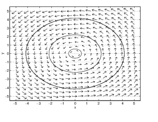
Centers

There is a new kind of solution that occurs only in centers — the time periodic solution — as we now explain. In Chapter ??, Theorem ?? we showed that when the $2\times 2$ matrix $C$ has purely eigenvalues $\pm i\tau$ with $\tau \neq 0$ , then $C$ is similar to the matrix $B = \mattwo {0}{-\tau }{\tau }{0}.$ In Table ??(b) we showed that solutions to $\dot {X}=BX$ are $X(t) = \mattwo {\cos (\tau t)}{-\sin (\tau t)}{\sin (\tau t)}{\cos (\tau t)}X_0 =R_{\tau t}X_0,$ where $X_0$ is the vector of initial conditions and $R_{\tau t}$ is a rotation matrix (recall (??) of Chapter ??).

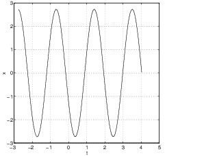
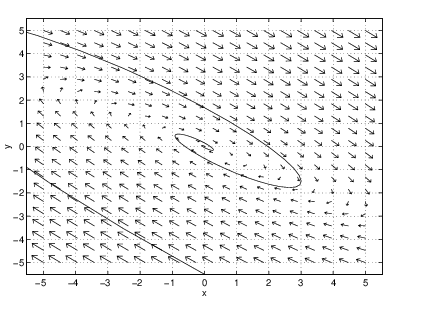
Note that every solution to $\dot {X}=BX$ traverses a circle around the origin as $R_{\tau t}$ rotates the plane counterclockwise through the angle $\tau t$ . As an example, we graph a solution to $\dot {X}=BX$ and its time series in Figure ?? when $\tau =3$ . All centers have nonzero trajectories that are either ellipses or circles, and those centers that do not have the form of $B$ typically produce ellipses as solutions. See Exercise ??.

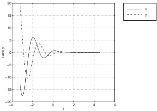
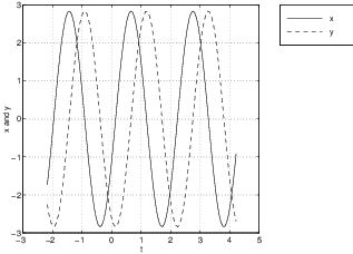
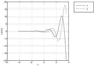
Figure 1: (Left) Solutions to $\dot {X}=BX$ for $\tau =3$ . (Right) Time series of a solution illustrating time periodicity.

It is instructive to see how solutions change when the real part of the eigenvalue traverses through zero. Suppose that $C$ has eigenvalues $\sigma \pm i\tau$ and is in normal form $C = \mattwo {\sigma }{-\tau }{\tau }{\sigma }.$ We illustrate this change by graphing the time series (of both $x$ and $y$ versus $t$ ) in Figure ?? with $\tau =3$ and $\sigma =-1,0,1$ , respectively. Note that when $\sigma <0$ the time series oscillate about zero but also damp down to zero, while when $\sigma >0$ the time series oscillate and diverge. When $\sigma = 0$ , there is an exact balance leading to time periodic solutions.

Figure 2: Solutions of $\dot {X}=BX$ for $\tau =3$ and $\sigma =-1,0,1$ .

Saddle Nodes

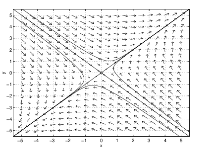
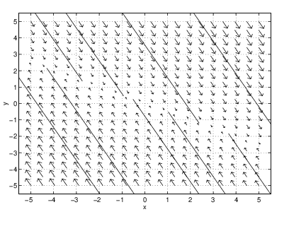
When the determinant of a matrix $C$ is zero, then $C$ must have a zero eigenvalue. The simplest way for $\det (C)$ to be zero is for $C$ to have a single zero eigenvalue. In this case we call the origin a saddle node.

So the eigenvalues of a saddle node are $\lambda _1=0$ and $\lambda _2\neq 0$ . For simplicity of discussion, we assume that $\lambda _2<0$ . Let $v_1$ and $v_2$ be the associated eigenvectors. Since $Cv_1=0$ , it follows that saddle nodes have a line of equilibria $X(t)=\alpha _1v_1$ for every scalar $\alpha _1$ .

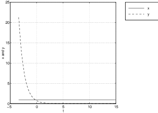
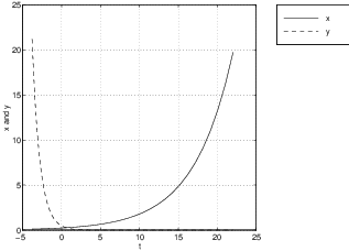
There is also a solution $X(t)=e^{\lambda _2 t}v_2$ that converges to the origin in forward time (since $\lambda _2<0$ ). The general solution to this system is $X(t) = \alpha _1 v_1 + \alpha _2 e^{\lambda _2 t}v_2,$ for scalars $\alpha _1$ and $\alpha _2$ . Since $\lambda _2<0$ this solution converges on the equilibrium $\alpha _1 v_1$ in forward time. Moreover, the trajectory for any solution stays for all time on the line parallel to the vector $v_2$ . The phase portrait for the system

$\begin{equation} \label{e:10ev} \frac{dX}{dt} = \mattwo{-2}{4}{1}{-2} X \end{equation}$ is shown in Figure ?? (left) along with the time series of a solution (right). Note how the time series (of $x$ versus $t$ ) asymptotes onto the $x$ coordinate of an equilibrium.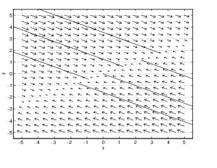

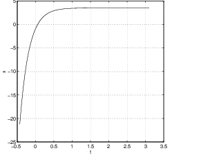
Figure 3: (Left) Phase portrait of (??). (Right) Time series of a solution.

The saddle-node is a nonhyperbolic equilibrium that sits between the hyperbolic saddle and the hyperbolic node (either the nodal sink or the nodal source), just as the center sits between the hyperbolic spiral source and the hyperbolic spiral sink. To illustrate this point we show three time series in Figure ?? for the system

$\begin{equation} \label{e:saddlenodebif} \frac{dX}{dt} = \mattwo{\mu}{0}{0}{-1}X \end{equation}$ when $\mu <0$ , $\mu =0$ , and $\mu >0$ . See how the $y$ time series decays exponentially to zero in forward time in each case. But the $x$ time series converges to zero when $\mu <0$ and grows exponentially when $\mu >0$ . Finally, when $\mu =0$ the $x$ time series is constant.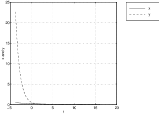

Figure 4: Time series for solutions of (??) when $\mu =-0.2,0,0.2$ .

Shears

The last example of a nonhyperbolic system occurs when the matrix $C$ has two zero eigenvalues — but only one linearly independent eigenvector. In this case we call the origin a shear. After a similarity transformation such a system is

$\begin{equation} \label{e:00} \frac{dX}{dt} = \mattwo{0}{1}{0}{0} X \end{equation}$ The solution is $(x(t),y(t)) = (x_0+y_0t,y_0).$ Thus solutions move along lines parallel to the $x$ axis through the point $(x_0,y_0)$ with speed $y_0$ . These trajectories move to the right when $y_0>0$ and to the left when $y_0<0$ .

Exercises

In Exercises ?? – ??, find a $2\times 2$ matrix $C$ so that the differential equation $\dot {X}=CX$ satisfies the given condition.

The origin is a center.

The origin is a saddle-node with equilibria on the line generated by the vector $(-1,2)$ .

Recall from Chapter ??, (??) that the undamped spring equation is $\frac {d^2x}{dt^2} + \kappa x = 0$ , where $\kappa >0$ .

As a first order system this equation is:
$\begin{eqnarray*} \dot{x} & = & y \\ \dot{y} & = & -\kappa x. \end{eqnarray*}$
Sketch the phase portrait of this equation.
The damped spring equation, written as a first order system, is:
$\begin{eqnarray*} \dot{x} & = & y \\ \dot{y} & = & -\kappa x-\sigma y, \end{eqnarray*}$
where $\sigma >0$ is the damping. Sketch the phase portrait of this equation.

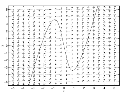
In Exercises ?? – ??, consider the four pictures in Figure ??. Each picture is a phase portrait of a system of differential equations $\dot {X}=CX$ where $C$ is a $2\times 2$ matrix. Answer the given question for each of these phase portraits.

What is the name of the type of equilibrium at the origin?

Is the origin asymptotically stable?

Is ${\rm trace}(C)$ positive, negative, or zero?

Is $\det (C)$ positive, negative, or zero?

Is ${\rm discriminant}(C)$ positive, negative, or zero?

(A) (B)

Figure 5: Phase portraits for planar linear systems in Exercises ?? – ??

In Exercises ?? – ??, consider the system of differential equations $\dot {X}=CX$ where $C$ is the given matrix. For each system determine whether the origin is hyperbolic or not and the type of equilibrium at the origin (spiral sink, center, etc.).

$C = \mattwo {1}{-1}{2}{1}$ .

$C = \mattwo {1}{1}{-1}{1}$ .

$C = \mattwo {3}{-1}{1}{1}$ .

$C = \mattwo {1}{1}{1}{1}$ .

$C = \mattwo {2}{-2}{4}{-2}$ .

$C = \mattwo {2}{2}{-2}{-2}$ .

$C = \mattwo {1}{1}{4}{1}$ .

Consider the system of differential equations $\dot {X}=CX$ where $C=\mattwo {2}{-10}{1}{-2}$ . By hand show that this system is a center and use pplane5 to determine its phase portrait. Describe both the similarities and the differences of the phase portrait of this system and the phase portrait in Figure ??.

Consider the system of differential equations $\dot {X}=CX$ where $C=\mattwo {2}{-4}{1}{-2}$ . By hand show that this system is a shear and use pplane5 to determine its phase portrait. Describe both the similarities and the differences of the phase portrait of this system and the phase portrait of (??).