Graphing Solutions to Differential Equations

$\newenvironment {prompt}{}{} \newcommand {\Sec }[2]{\section {#1}} \newcommand {\trademark }[0]{{R\!\!\!\!\!\bigcirc }} \newcommand {\EXER }[0]{\section *{Exercises}} \newcommand {\CEXER }[0]{} \newcommand {\TEXER }[0]{} \newcommand {\R }[0]{\mbox {$\Bbb {R}$}} \newcommand {\C }[0]{\mbox {$\Bbb {C}$}} \newcommand {\Z }[0]{\mbox {$\Bbb {Z}$}} \newcommand {\N }[0]{\mbox {$\Bbb {N}$}} \newcommand {\D }[0]{\mbox {{\bf D}}} \newcommand {\setmin }[0]{\;\mbox {--}\;} \newcommand {\Matlab }[0]{{M\small {AT\-LAB}} } \newcommand {\Matlabp }[0]{{M\small {AT\-LAB}}} \newcommand {\computer }[0]{\Matlab Instructions} \newcommand {\half }[0]{\mbox {$\frac {1}{2}$}} \newcommand {\compose }[0]{\raisebox {.15ex}{\mbox {{\scriptsize $\circ $}}}} \newcommand {\AND }[0]{\quad \mbox {and}\quad } \newcommand {\vect }[2]{\left (\begin {array}{c} #1_1 \\ \vdots \\ #1_{#2}\end {array}\right )} \newcommand {\mattwo }[4]{\left (\begin {array}{rr} #1 & #2\\ #3 &#4\end {array}\right )} \newcommand {\mattwoc }[4]{\left (\begin {array}{cc} #1 & #2\\ #3 &#4\end {array}\right )} \newcommand {\vectwo }[2]{\left (\begin {array}{r} #1 \\ #2\end {array}\right )} \newcommand {\vectwoc }[2]{\left (\begin {array}{c} #1 \\ #2\end {array}\right )} \newcommand {\inv }[0]{^{-1}} \newcommand {\CC }[0]{{\cal C}} \newcommand {\CCone }[0]{\CC ^1} \newcommand {\Span }[0]{{\rm span}} \newcommand {\rank }[0]{{\rm rank}} \newcommand {\trace }[0]{{\rm tr}} \newcommand {\RE }[0]{{\rm Re}} \newcommand {\IM }[0]{{\rm Im}} \newcommand {\nulls }[0]{{\rm null\;space}} \newcommand {\dps }[0]{\displaystyle } \newcommand {\arraystart }[0]{\renewcommand {\arraystretch }{1.8}} \newcommand {\arrayfinish }[0]{\renewcommand {\arraystretch }{1.2}} \newcommand {\Start }[1]{\vspace {0.08in}\noindent {\bf Section~\ref {#1}}} \newcommand {\exer }[1]{\noindent {\bf \ref {#1}}} \newcommand {\ans }[0]{} \newcommand {\matthree }[9]{\left (\begin {array}{rrr} #1 & #2 & #3 \\ #4 & #5 & #6 \\ #7 & #8 & #9\end {array}\right )} \newcommand {\cvectwo }[2]{\left (\begin {array}{c} #1 \\ #2\end {array}\right )} \newcommand {\cmatthree }[9]{\left (\begin {array}{ccc} #1 & #2 & #3 \\ #4 & #5 & #6 \\ #7 & #8 & #9\end {array}\right )} \newcommand {\vecthree }[3]{\left (\begin {array}{r} #1 \\ #2 \\ #3\end {array}\right )} \newcommand {\cvecthree }[3]{\left (\begin {array}{c} #1 \\ #2 \\ #3\end {array}\right )} \newcommand {\cmattwo }[4]{\left (\begin {array}{cc} #1 & #2\\ #3 &#4\end {array}\right )} \newcommand {\thehelp }[0]{\thesection .\arabic {equation}} \newcommand {\matlabEquation }[0]{\let \oldtheequation \theequation \renewcommand {\theequation }{\oldtheequation *}\begin {equation}} \newcommand {\HyperFirstAtBeginDocument }[0]{\AtBeginDocument } \newcommand {\epstopdfsetup }[0]{\setkeys {ETE}} changed the theorem header of amsthm failed\MessageBreak }}} \newcommand {\GetTitleStringSetup }[0]{\setkeys {gettitlestring}} \newcommand {\Sectionformat }[2]{#1}$ $% This file was *autogenerated* from graphingSolutionsToDifferentialEquations.sagetex.sage with % sagetex.py version 2015/08/26 v3.0-92d9f7a %4458fb43d23abeea866ec3b50d7e2dd1% md5sum of corresponding .sage file (minus "goboom","current_tex_line",and pause/unpause lines)$

Solutions to differential equations can be graphed in several different ways, each giving different insight into the structure of the solutions. We begin by asking what object is to be graphed. Do we first solve the differential equation and then graph the solution, or do we let the computer find the solution numerically and then graph the result? The first method assumes that we can find a formula for the solution (such as $x(t)=x_0e^{\lambda t}$ ). A solution to a differential equation for which we have an explicit formula is called a closed form solution. Using MATLAB we can graph closed form solutions, as we showed in Figure ??. The second method of graphing solutions requires having a numerical method that can numerically integrate the differential equation to any desired degree of accuracy.

In fact, there are rather few differential equations that can be solved in closed form (though the linear systems that we describe in this chapter are ones that can be solved in closed form). Without formulas, the first method is impossible. There are, however, several efficient algorithms for the numerical solution of (systems of) ordinary differential equations and these methods have been preprogrammed in MATLAB. In our discussions, we treat MATLAB as a black box numerical integration solver of ordinary differential equations.

A Single First Order Ordinary Differential Equation

We begin our discussion of the numerical integration of differential equations with the single first order differential equation of the form:

$\begin{equation} \label{nonaut} \frac{dx}{dt}(t) = f(t,x(t)). \end{equation}$ The equation is first order since only the first derivative of the function $x(t)$ appears in the equation. If the second derivative appeared in the equation, then the equation would be a second order equation.

Independent ( $t$ ) and Dependent ( $x$ ) Variables

Sometimes this equation is also written in the form

$\begin{equation} \label{nonaut2} \frac{dx}{dt} = f(t,x) \end{equation}$ and in this form both $t$ and $x$ appear as variables. But $x$ is a function $x(t)$ depending on $t$ , and therefore the variable $t$ is called the independent variable, while the variable $x$ is called the dependent variable.

Autonomous versus Nonautonomous

When the right hand side $f$ does not depend explicitly on the independent time variable $t$ , then the equation is called autonomous. More explicitly, in (??), the differential equation is autonomous when $f(t,x)=g(x)$ . Equation (??) is an example of an autonomous differential equation since $f(t,x)=\lambda x$ .

When $f$ depends explicitly on the independent time variable $t$ , the differential equation is called nonautonomous. Suppose in our example of interest rates in Section ?? we had assumed that the interest rate $r$ changes in time. In such a case we would write $r=r(t)$ and the differential equation modeling how the principal $P(t)$ changes in time would be written as

$\begin{equation} \label{E:varinterest} \frac{dP}{dt} = r(t)P. \end{equation}$ This equation is an example of a nonautonomous differential equation since $f(t,P) = r(t)P$ . For instance, suppose that at time $t=0$ the principal in our account is $P_0$ , and the interest rate is $5.5\$ . Now suppose the bank changes the interest rate after six months to $4.5\$ . Then $P(t)$ is a solution to (??), where $r(t) = \left \{\begin {array}{l} 0.055\quad \mbox {for $0\le t < 0.5$, and}\\ 0.045\quad \mbox {for $0.5\le t$,} \end {array}\right .$ and $P(0)=P_0$ .

Another example of a nonautonomous differential equation is given by

$\begin{equation} \label{dfeq} \frac{dx}{dt} = x^2-t. \end{equation}$

Time Series and Phase Space Plots

There are two different methods for visualizing the result of numerical integration of differential equations of the form (??): time series plots and phase space plots. These two methods are based on interpreting the derivative $dx/dt$ alternatively as either the slope of a tangent line or as the velocity of a particle.

A time series plot for a solution to (??) is found by plotting $x$ versus $t$ as we did for the closed form solution in Figure ??. However, when graphing time series of solutions we do not need to find closed form solutions. To understand how this is done, we briefly discuss what equation (??) is actually saying about a solution $x(t)$ . This equation states that the slope of the tangent line to the graph of the function $x(t)$ at time t ( $dx/dt$ ) is known and equals $f(t,x(t))$ . Thus we can use the right hand side of (??) to draw the tangent lines to $x(t)$ at each point in the $tx$ -plane. This leads to the notion of a line field. The rough idea behind the numerical integration scheme is to fit a curve $(t,x(t))$ into the $tx$ -plane in such a way that the tangent lines to the curve match the tangent lines specified by the slope $f$ .

A phase space plot is based on the other interpretation of a derivative as a rate of change — a velocity. We let $x(t)$ denote the position of a particle on the real line at time $t$ . The function $f(t,x)$ denotes the velocity of that particle when the particle is at position $x$ at time $t$ . Thus, to view the phase space plot, we need to see the particle moving along the real line; that is, we need to see how $x(t)$ changes in $t$ . Later, we will use MATLAB graphics to actually visualize the particle movement.

Thus time series are graphs of functions in the $tx$ -plane while phase space plots are graphs on the real line $x$ . We discuss time series plots in this section and phase line plots in the next.

Line Fields

We begin our discussion of line fields (or synonymously direction fields) by focusing on the information about solutions that can directly be extracted from the equation itself. To illustrate this we consider the differential equation (??).

As mentioned, the differential equation $\dot {x}=x^2-t$ reflects the fact that the value of the derivative of a solution $x(t)$ at time $t$ is given by $(x(t))^2-t$ . In other words, the slope of the tangent line to the solution is known and is given by the right hand side of the differential equation.

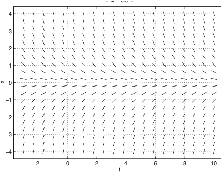
We can use this information to sketch all the tangent lines at each point $(t_0,x_0)$ of a rectangle in the $tx$ -plane. We do this by drawing a small line segment at each point with the slope determined by the right hand side. In this way we obtain the line field. In Figure ?? we show a line field corresponding to the differential equation (??).

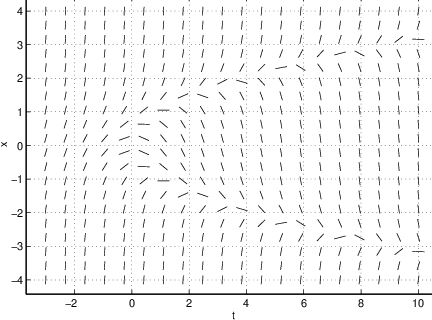
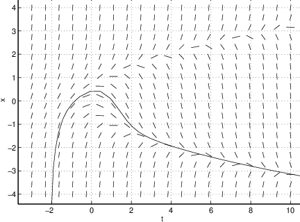
Figure 1: Left: Line field for (??) for $t\in [-3,10]$ and $x\in [-4,4]$ . Right: a solution starting for $t=-2$ at $x(-2)=-4$ .

By looking at the left hand image in Figure ?? we can imagine how solution curves fit into the diagram; indeed, we can almost use this line field to make freehand sketches of solutions to (??). The right hand image in Figure ?? shows the solution starting at the initial condition $x(-2) = -4$ , which is the point $(x,t)=(-4,-2)$ .

Graphing Solutions Using dfield5

We now explain how to use MATLAB to display the graphs of solutions to the differential equation (??) for different choices of initial conditions. It is a tedious process to use MATLAB directly to both compute and graphically display these solutions. Instead, we use a program written in MATLAB by John Polking for graphing both the line field and the time series of a solution to any ordinary differential equation of the form (??). In MATLAB this program is addressed by typing

dfield5

In response, a window appears with the title DFIELD5 Setup. The differential equation under consideration is displayed in the upper big grey frame. In this case it is $x' = x^2 - t,$ which is (??). Now use the left mouse button to click onto the button Proceed. Then another window, having the title DFIELD5 Display, appears. In this window, one should see the line field shown in Figure ??. We may compute the solution going through the point $(t_0,x_0)=(-2,-4)$ in the $(t,x)$ -plane by clicking on that point with any mouse button. dfield5 should reproduce the right hand side in Figure ??.

Suppose that we want to solve numerically equation (??) using dfield5. To enter this equation with $\lambda = 0.5$ , we have to change the setup. Begin by clicking into the window where the right hand side x2–t can be found and then replace it by 0.5*x. Now use the left mouse button to click onto the button Proceed. In the window titled DFIELD5 Display, one should see the line field shown on the left in Figure ??.

Figure 2: Left: Line field for $\dot {x}=0.5x$ for $t\in [-4,10]$ and $x\in [-4,4]$ . Right: A solution starting at $t=0$ and $x>0$ but small.

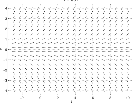
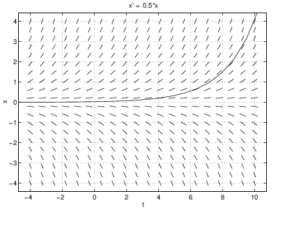
Now we may compute solutions going through a certain point $(t_0,x_0)$ in the $(t,x)$ -plane by clicking with any mouse button on that point. The solution is then computed first in forward time and then in backward time. For example, if we click on a point near $t=x=0$ where $x>0$ , dfield5 produces the solution shown on the right in Figure ??. Note the similarity with the graph of the closed form solution in Figure ?? when $\lambda =0.5$ .

By clicking several times it appears that all solutions diverge to either plus or minus infinity as $t$ goes to infinity. Indeed, by (??) we know that the solutions are of the form $x(t) = x_0 e^{0.5 t}$ , and hence this behavior is expected for $x_0\not = 0$ . To compute a solution corresponding to the case when $x_0=0$ , we bring up the menu DFIELD5 Options and select Keyboard input. This allows us to type in the initial values $t=-2$ and $x=0$ . The action Compute then leads to the computation of the solution $x(t)=0$ corresponding to $x_0=0$ .

The value of $\lambda =0.5$ can be changed by editing the corresponding window in the DFIELD5 Setup. For instance, if we replace the $0.5$ by $-0.8$ and push Proceed, then the current line field is replaced by the line field shown in Figure ??.

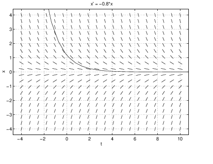
Figure 3: Left: Line field for $\dot {x}=-0.8 x$ for $t\in [-4,10]$ and $x\in [-4,4]$ . Right: A solution starting at $t=0$ and $x$ between $1$ and $2$ .

By computing different solutions, it seems as though all of them converge to zero as $t$ goes to infinity, which agrees with (??).

Autonomous and Nonautonomous Equations in dfield5

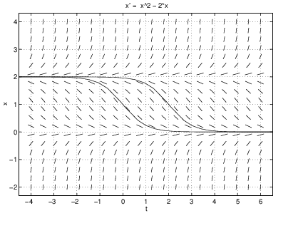
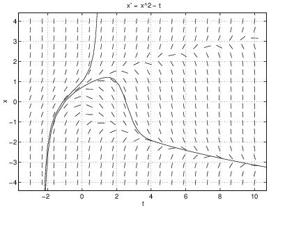
In a sense, solutions of autonomous equations do not depend on the initial time $t_0$ , but just on the initial position $x_0$ . More precisely, let $x_1(t)$ be the solution to $\frac {dx}{dt} = f(x)$ with initial condition $x(0)=x_0$ and let $x_2(t)$ be a solution to the same differential equation with initial condition $x(t_0)=x_0$ . Then

$\begin{equation} \label{E:initdiff} x_2(t) = x_1(t-t_0). \end{equation}$ This statement can be verified by noting that the definition of $x_2(t)$ in (??) satisfies the initial value $x_2(t_0)=x_1(t_0-t_0)=x_1(0)=x_0,$ and, using the chain rule, the differential equation $\frac {dx_2}{dt}(t) = \frac {dx_1}{dt}(t-t_0) = f(x_1(t-t_0))=f(x_2(t)).$ So the solution $x_2(t)$ is the same as the solution $x_1(t)$ with just a shift in time $t$ . In general, the same statement is not true for nonautonomous equations.

This difference between autonomous and nonautonomous equations can be visualized using dfield5. On the left in Figure ?? we graph two solutions of the autonomous differential equation $\dot {x}=x^2-2x$ with initial conditions $x(0)=1$ and $x(2)=1$ . Note that one solution is obtained from the other just by shifting by two time units. On the right of that figure we graph two solutions of the nonautonomous differential equation $\dot {x}=x^2-t$ with initial conditions $x(0)=1$ and $x(2)=1$ . Note that the two solutions are most definitely not obtained one from the other by a time shift.

Figure 4: Left: Solutions of the autonomous equation $\dot {x}=x^2-2x$ with initial conditions $x(0)=1$ and $x(2)=1$ . Right: Solution of the nonautonomous differential equation $\dot {x}=x^2-t$ with initial conditions $x(0)=1$ and $x(2)=1$ .

Exercises

In Exercises ?? – ?? determine whether the solution to the given differential equation with given initial condition is increasing or decreasing at the initial point.

ODE: $\dot {x}=x-t$ ; initial condition: $x(1)=2$ .

ODE: $\dot {x}=x-t$ ; initial condition: $x(2)=1$ .

ODE: $\dot {x}=x^2-tx$ ; initial condition: $x(1)=2$ .

ODE: $\dot {x}=x^2-tx-t$ ; initial condition: $x(2)=-1$ .

In Exercises ?? – ?? sketch by hand the line field of the given differential equation on the given rectangle.

ODE: $\dot {x}=x-t$ ; rectangle: $0\leq x\leq 2; -1\leq t\leq 1$ .

ODE: $\dot {x}=x+t$ ; rectangle: $-2\leq x\leq 2; -1\leq t\leq 2$ .

ODE: $\dot {x}=xt$ ; rectangle: $-1\leq x\leq 1; -1\leq t\leq 1$ .

ODE: $\dot {x}=x/t$ ; rectangle: $0< x\leq 2; 0< t\leq 2$ .

In Exercises ?? – ?? determine whether the given differential equation is autonomous or nonautonomous.

$\dot {x}=x-t$ .

$\dot {x}=x^2-x$ .

$\dot {x}=x\sin (x)$ .

$\dot {x}=x\cos (t)$ .

In Exercises ?? – ?? use dfield5 to compute several solutions to the given differential equations in the specified region.

$\dot {x} = xt$ , $t\in [0,2]$ , $x\in [-1,1]$ .

$\dot {x} = tx^2$ , $t\in [0,4]$ , $x\in [-4,4]$ .

$\dot {x} = x-\sin (t)$ , $t\in [-2,10]$ , $x\in [-4,4]$ .

Compute $x(2)$ , where $x(t)$ is the solution to the differential equation $\dot {x} = 0.6x$ with initial condition $x(0)=0.5$ , in two different ways, as follows:

Use Keyboard input in dfield5 to compute the solution with initial value $x(0)=0.5$ . Use the zoom in feature in the DFIELD5 Edit menu to compute $x(2)$ to an accuracy of two decimal places. (Drag a rectangle around the point you are interested in. Repeat this several times until you can read off the value $x(2)$ of the solution.)
Use MATLAB to compute the value of the exact solution of the form (??) with initial value $x(0)=0.5$ .
Is your answer obtained using dfield5 in (a) accurate to within two decimal places of the answer obtained using (b)? If not, which answer do you trust more, and why?

Use dfield5 to compute solutions to the differential equation $\dot {x} = x^2-tx+2t$ . Use Keyboard input to compute the solution with initial value $x(-1)=-1$ . What is the minimum value of this solution $x(t)$ on the interval $-2\leq t\leq 1$ ? Plot solutions to this equation starting with at least six or seven different initial conditions. Then print the result.

Use dfield5 to compute solutions to the differential equation $\begin{equation} \label{E:freehand} \dot{x} = x^3-2t^2x-t. \end{equation}$ Print the line field of (??) on the intervals $t\in [-2,2]$ and $x\in [-2,3]$ . Use the line field to draw freehand the solution to (??) starting at $(t_0,x_0)=(-2,1)$ . Then set the initial condition using Keyboard input and print the numerically computed solution. Finally, compare your freehand drawing with the numerically computed result.

Draw the direction field for $\begin{equation} \label{ex:at} \frac{dx}{dt} = \frac{x}{x-t}. \end{equation}$ Assuming that $x(2)=3$ , estimate $x(137)$ .
Verify that $x(t) = t + \sqrt {t^2-3}$ is the solution to (??). Then show that $x(t)$ satisfies the initial condition $x(2)=3$ .
Compare your estimate of the solution to (??) obtained using dfield5 with the exact solution $x(137)= 137 +\sqrt {18766} \approx 273.989$