Separation of Variables

$\newenvironment {prompt}{}{} \newcommand {\Sec }[2]{\section {#1}} \newcommand {\trademark }[0]{{R\!\!\!\!\!\bigcirc }} \newcommand {\EXER }[0]{\section *{Exercises}} \newcommand {\CEXER }[0]{} \newcommand {\TEXER }[0]{} \newcommand {\R }[0]{\mbox {$\Bbb {R}$}} \newcommand {\C }[0]{\mbox {$\Bbb {C}$}} \newcommand {\Z }[0]{\mbox {$\Bbb {Z}$}} \newcommand {\N }[0]{\mbox {$\Bbb {N}$}} \newcommand {\D }[0]{\mbox {{\bf D}}} \newcommand {\setmin }[0]{\;\mbox {--}\;} \newcommand {\Matlab }[0]{{M\small {AT\-LAB}} } \newcommand {\Matlabp }[0]{{M\small {AT\-LAB}}} \newcommand {\computer }[0]{\Matlab Instructions} \newcommand {\half }[0]{\mbox {$\frac {1}{2}$}} \newcommand {\compose }[0]{\raisebox {.15ex}{\mbox {{\scriptsize $\circ $}}}} \newcommand {\AND }[0]{\quad \mbox {and}\quad } \newcommand {\vect }[2]{\left (\begin {array}{c} #1_1 \\ \vdots \\ #1_{#2}\end {array}\right )} \newcommand {\mattwo }[4]{\left (\begin {array}{rr} #1 & #2\\ #3 &#4\end {array}\right )} \newcommand {\mattwoc }[4]{\left (\begin {array}{cc} #1 & #2\\ #3 &#4\end {array}\right )} \newcommand {\vectwo }[2]{\left (\begin {array}{r} #1 \\ #2\end {array}\right )} \newcommand {\vectwoc }[2]{\left (\begin {array}{c} #1 \\ #2\end {array}\right )} \newcommand {\inv }[0]{^{-1}} \newcommand {\CC }[0]{{\cal C}} \newcommand {\CCone }[0]{\CC ^1} \newcommand {\Span }[0]{{\rm span}} \newcommand {\rank }[0]{{\rm rank}} \newcommand {\trace }[0]{{\rm tr}} \newcommand {\RE }[0]{{\rm Re}} \newcommand {\IM }[0]{{\rm Im}} \newcommand {\nulls }[0]{{\rm null\;space}} \newcommand {\dps }[0]{\displaystyle } \newcommand {\arraystart }[0]{\renewcommand {\arraystretch }{1.8}} \newcommand {\arrayfinish }[0]{\renewcommand {\arraystretch }{1.2}} \newcommand {\Start }[1]{\vspace {0.08in}\noindent {\bf Section~\ref {#1}}} \newcommand {\exer }[1]{\noindent {\bf \ref {#1}}} \newcommand {\ans }[0]{} \newcommand {\matthree }[9]{\left (\begin {array}{rrr} #1 & #2 & #3 \\ #4 & #5 & #6 \\ #7 & #8 & #9\end {array}\right )} \newcommand {\cvectwo }[2]{\left (\begin {array}{c} #1 \\ #2\end {array}\right )} \newcommand {\cmatthree }[9]{\left (\begin {array}{ccc} #1 & #2 & #3 \\ #4 & #5 & #6 \\ #7 & #8 & #9\end {array}\right )} \newcommand {\vecthree }[3]{\left (\begin {array}{r} #1 \\ #2 \\ #3\end {array}\right )} \newcommand {\cvecthree }[3]{\left (\begin {array}{c} #1 \\ #2 \\ #3\end {array}\right )} \newcommand {\cmattwo }[4]{\left (\begin {array}{cc} #1 & #2\\ #3 &#4\end {array}\right )} \newcommand {\thehelp }[0]{\thesection .\arabic {equation}} \newcommand {\matlabEquation }[0]{\let \oldtheequation \theequation \renewcommand {\theequation }{\oldtheequation *}\begin {equation}} \newcommand {\HyperFirstAtBeginDocument }[0]{\AtBeginDocument } \newcommand {\epstopdfsetup }[0]{\setkeys {ETE}} changed the theorem header of amsthm failed\MessageBreak }}} \newcommand {\GetTitleStringSetup }[0]{\setkeys {gettitlestring}} \newcommand {\Sectionformat }[2]{#1}$ $% This file was *autogenerated* from separationOfVariables.sagetex.sage with % sagetex.py version 2015/08/26 v3.0-92d9f7a %18766d3678f7a8d76180810c8c138c77% md5sum of corresponding .sage file (minus "goboom","current_tex_line",and pause/unpause lines)$

In this section we discuss a method for finding closed form solutions to a particular class of nonautonomous first order ordinary differential equations

$\begin{equation} \label{e:nonauto} \frac{dx}{dt} = f(t,x). \end{equation}$ These particular equations are separable equations having the form $\begin{equation} \label{eq:gh} \frac{dx}{dt} = g(x) h(t), \end{equation}$ where $g,h:\R \to \R$ are continuous functions. There are two special cases of (??): the case $g(x)=1$ and the case $h(t)=1$ .

The Special Case $g(x)=1$ : Integration Theory

The assumption that $g(x)=1$ in (??) leads to the differential equation

$\begin{equation} \label{e:g=1} \frac{dx}{dt} = h(t). \end{equation}$ In Section ?? we saw that this differential equation is easily solved by direct integration. For example, if $h(t)=t^2$ then the solution to (??) with initial condition $x(2)=5$ is found as follows. By direct integration, $x(t) = \int t^2 dt = \frac {1}{3}t^3 + C.$ It then follows that $x(2) = \frac {8}{3} + C = 5;$ so $C = 5 - \frac {8}{3} = \frac {7}{3}.$

The Special Case $h(t)=1$ : Autonomous Equations

The second special case in (??) leads to the autonomous differential equation

$\begin{equation} \label{e:h=1} \frac{dx}{dt} = g(x). \end{equation}$ Begin by noting that equilibria are special solutions to (??) that we can find by solving the equation $g(x)=0$ . More precisely, if $g(x_0)=0$ , then $x(t)=x_0$ is a constant solution to (??).

We find the nonequilibrium solutions by direct integration — but only after using change of variables in integration. To solve (??), just divide both sides of this equation by $g(x)$ , obtaining $\frac {1}{g(x)}\frac {dx}{dt} = 1,$ and integrate with respect to $t$ , obtaining $\int \frac {1}{g(x)} \frac {dx}{dt} dt = \int dt + C = t + C.$ After substituting $y=x(t)$ and using the chain rule, the integral on the left becomes $\int \frac {1}{g(y)}dy.$ Replacing $y$ by $x$ , we obtain $\int \frac {1}{g(x)}dx = t + C.$

As a simple example, solve the growth rate equation (??)

$\begin{equation} \label{lin1a} \frac{dx}{dt} = \lambda x \end{equation}$ using this technique of integration. It follows that $\int \frac {1}{x}dx = \lambda t + C.$ So, to solve (??), we need to know how to integrate the function $1/x$ . Recalling that this integral is just $\ln |x|$ we obtain $\ln |x(t)| = \lambda t + C.$ We solve this equation by exponentiation, obtaining $|x(t)| = K e^{\lambda t},$ where $K = e^C \geq 0$ . On dropping the absolute value signs, we obtain $x(t) = K e^{\lambda t},$ for arbitrary $K$ . Of course, this is precisely the solution that we found in (??).

It is worth reflecting on the information from calculus that we needed to solve (??). In Section ?? we found the solution to this equation by asking what function has a derivative that is a multiple of itself. We then had to remember that $e^{\lambda t}$ is such a function and then prove that up to the constant $K$ this was the only such function (recall Theorem ??). Here we needed to remember the indefinite integral of $1/x$ and then solve for $x$ in terms of $t$ .

We now summarize this technique for solving the autonomous differential equation (??). Let $G(x)$ be an indefinite integral of $1/g(x)$ . Then, after division by $g(x)$ , integrating both sides of (??) with respect to $t$ leads to the equation $G(x) = t + C.$ Then we need to solve this algebraic equation for $x$ in terms of $t$ . This last step is often quite difficult, as we show by example below.

There is one additional point that needs to be remembered when using this technique. The constant $C$ is, as usual, related to an initial condition. Indeed, if we wish to solve (??) with the initial condition $x(t_0)=x_0$ , then we can solve for $C = G(x_0) - t_0.$

An Example of Blow-up in Finite Time

Consider the nonlinear differential equation

$\begin{equation} \label{e:x^2} \frac{dx}{dt} = x^2 \end{equation}$ satisfying the initial condition $x(t_0)=x_0$ . Using the preceding discussion, we can solve (??) by integration. Specifically, on division we obtain $\frac {1}{x^2}\frac {dx}{dt} = 1,$ and on integration with respect to $t$ , we obtain $-\frac {1}{x} = t + C.$ Solving for $x$ in terms of $t$ we obtain $x(t) = - \frac {1}{t+C}.$ Finally, use the initial condition to solve for $C$ . On substitution $x_0 = x(t_0) = - \frac {1}{t_0+C}.$ Hence $C = -\frac {1}{x_0} - t_0,$ which is fine unless $x_0$ happens to equal $0$ . However, in that case, we have just recovered the equilibrium solution $x(t)=0$ .

On setting $K = \frac {1}{x_0}+t_0,$ we obtain the solution $x(t) = \frac {1}{K-t}.$ For example, if $t_0=0.1$ and $x_0=2$ , then $K=0.6$ and

$\begin{equation} \label{E:solnx^2} x(t) = \frac{1}{0.6-t}. \end{equation}$

Example (??) shows that solutions to nonlinear differential equations possess qualitative properties that are different from those of the linear equation $\dot {x}=\lambda x$ . In particular:

Solutions can approach infinity in finite time. For example, the solution (??) with initial condition $x(0.1)=2$ goes to infinity as $t$ approaches $0.6$ .
Solutions may not be defined for all $t\in \R$ . Indeed, the solution (??) has a singularity at $t=0.6$ and is defined for either $t> 0.6$ or $t<0.6$ .

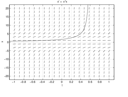
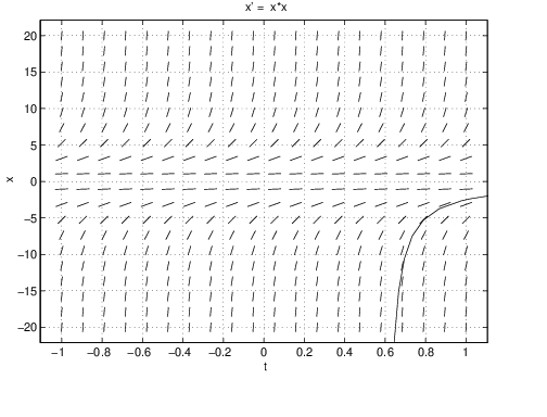
We can solve equation (??) using dfield5. Using Keyboard input set the initial condition at $(x_0,t_0)=(2,0.1)$ and obtain the trajectory in Figure ??(left). Note that this solution goes to infinity in forward time while approaching $t=0.6$ . Now set the initial condition to $(x_0,t_0)=(1,-2.5)$ and see that the solution goes to negative infinity as $t$ approaches $0.6$ from above. See Figure ??(right). Finally note that both of these solutions are given by the same formula (??).

Figure 1: Solutions using dfield5 for $\frac {dx}{dt} = x^2$ with initial conditions: (left) $(x_0,t_0)=(2,0.1)$ and (right) $(x_0,t_0)=(1,-2.5)$ .

An Example that Cannot be Solved in Closed Form

Consider the differential equation

$\begin{equation} \label{E:ncf} \frac{dx}{dt} = \frac{x}{x-1} \end{equation}$ with initial condition $x(1)=2$ . On division (??) becomes $\left (1-\frac {1}{x}\right )\frac {dx}{dt} = 1.$ Integration with respect to $t$ yields $x - \ln |x| = t + C.$ Using the initial condition, we see that $C = 2 - \ln 2 -1 = 1 - \ln 2.$ Note that for $t$ near $1$ , the initial condition implies that $x(t)>0$ . Hence $x(t)$ satisfies $\begin{equation} \label{e:solnncf} x -\ln x = t + 1 - \ln 2. \end{equation}$ Unfortunately, this equation cannot be solved explicitly for $x$ as a function of $t$ ; that is, there is no closed form solution for $x(t)$ . Nevertheless, $x(t)$ is defined implicitly by (??). This equation can, however, be solved numerically by dfield5 just as easily as equations that have closed form solutions. See Exercise ??.

The General Solution by Separation of Variables

The solution to the initial value problem for the separation of variables equation

$\begin{equation} \label{eq:ghivp} \dps \frac{dx}{dt} = g(x) h(t), \end{equation}$ where $x(t_0) = x_0$ , is obtained by combining the integrations of the two special cases just considered.

Note that if $g(x_0)=0$ , then $x(t)=x_0$ is an equilibrium solution to (??). So we can assume

$\begin{equation} \label{eq:gx0} g(x_0)\not=0, \end{equation}$ and divide (??) by $g(x)$ to obtain $\frac {1}{g(x)}\frac {dx}{dt}= h(t).$ Integrating with respect to $t$ yields $\int \frac {1}{g(x)} \frac {dx}{dt}dt = \int h(t) dt + C.$ As before, on changing variables, we obtain $\int \frac {1}{g(x)} dx = \int h(t) dt.$ Thus, the abstract solution to (??) can be written as $\begin{equation} \label{E:G=H+K} G(x) = H(t) + C, \end{equation}$ where $G$ is an indefinite integral of $1/g$ and $H$ is an indefinite integral of $h$ , and $\begin{equation} \label{E:G=H+Kinit} C = G(x_0)-H(t_0). \end{equation}$

An Example Solving the Initial Value Problem

We illustrate the technique of separation of variables with the following example. Find the solution of the initial value problem $\frac {dx}{dt} = \frac {t}{x^2}$ where $x(1)=2$ . Here $g(x) = 1/x^2$ and $h(t) = t$ , so that $G(x)=\int x^2 dx= \frac {1}{3}x^3 \AND H(t) = \int t dt = \frac {1}{2}t^2.$ Since $t_0=1$ and $x_0=2$ , we can use (??) to see that $C = G(2)-H(1) = \frac {8}{3} -\frac {1}{2} = \frac {13}{6},$ and (??) to see that the solution $x(t)$ satisfies $\frac {1}{3}x(t)^3 = \frac {1}{2}t^2 + \frac {13}{6}.$ Therefore, $x(t) = \left (\frac {3t^2+13}{2}\right )^{1/3}.$ The reader may check that this function is indeed a solution satisfying the specified initial condition.

An Example Finding a General Solution

With this example, we illustrate how to use separation of variables to find all solutions of a differential equation in the form (??). Consider

$\begin{equation} \label{eq:x1t2} \frac{dx}{dt} = \frac{(x+1)(t^2+1)}{t} \end{equation}$ for $t>0$ . Using our notation we have $g(x) = x+1 \AND h(t) = t+\frac {1}{t}.$ Note that $g(-1)=0$ and hence that $x(t)=-1$ is the constant equilibrium solution to (??). For all the other initial conditions, we obtain $G(x)=\int \frac {1}{x+1} dx = \ln |x+1| \AND H(t) = \int \left (t + \frac {1}{t}\right )dt = \frac {1}{2}t^2 + \ln |t|.$ Thus, in this example, identity (??) implies that the solution $x(t)$ satisfies $\ln |x(t)+1| = \frac {1}{2}t^2 + \ln |t| + C.$ Hence $|x(t)+1| = K|t|e^{t^2/2},$ for some constant $K>0$ and nonconstant solutions of (??) are in one-to-one correspondence with functions $x(t) = Kte^{t^2/2}-1$ for $K\in \R$ . Note that setting $K=0$ recovers the constant solution $x(t)=-1$ .

Exercises

In Exercises ?? – ?? decide whether or not the method of separation of variables can be applied to the given differential equation. If this method can be applied, then specify the functions $g$ and $h$ — but do not perform the integrations.

$\dps \frac {dx}{dt} = x^{1/2}\cos t$ .

$\dps \frac {dx}{dt} = (x+xt)\tan x$ .

$\dps \frac {dx}{dt} = (x+t)(x-t)$ .

$\dps \frac {dx}{dt} = 3-2x+3t-2xt$ .

In Exercises ?? – ?? solve the given initial value problem by separation of variables.

$\dps \frac {dx}{dt} = -3x,\quad x(0)=-1.$

$\dps \frac {dx}{dt} = \frac {t^3-1}{\cos x}, \quad x(\pi )=\frac {\pi }{2}.$

$\dps \frac {dx}{dt} = 2\sqrt {tx},\quad x(1)=1.$

In Exercises ?? – ?? use separation of variables to find all the solutions of the given differential equation.

$\dps \frac {dx}{dt} = 2x$ .

$\dps \frac {dx}{dt} = 5x+2$ .

$\dps \frac {dx}{dt} = \frac {\sin t}{x}$ .

We have studied the autonomous linear differential equation $\dot {x}=\lambda x$ when $\lambda \neq 0$ and have shown that solutions exist for all time and tend either to $0$ or to $\pm \infty$ as $t\to \pm \infty$ . See (??) and Figure ??. In Exercises ?? – ?? explore the behavior of solutions $x(t)$ of the given nonlinear (and often nonautonomous) differential equation using dfield5. Where possible, describe the differences between the behavior of solutions of the given differential equation and the linear differential equation.

Hint: Here is a list of properties of solutions that are not valid for solutions to the linear differential equation:

Solutions blow up in finite time (that is, $\lim _{t\to t_0}x(t)=\pm \infty$ ).
Solutions do not exist for all time.
Multiple solutions are bounded in both forward and backward time. (In the linear system only the zero solution $x(t)=0$ is bounded in both forward and backward time.)
Solutions stop (that is, solutions limit in either forward or backward time on a finite value of $x$ in finite time $t$ ).

Use dfield5 to determine which of these properties of solutions are valid for the given differential equations. Also, when exploring Exercises ?? – ?? be prepared to use the Stop button in the DFIELD5 Display window to stop the numerical integration.

$\dps \frac {dx}{dt} = \frac {1}{x}$ .

$\dps \frac {dx}{dt} = \frac {1}{tx}$ .

$\dps \frac {dx}{dt} = \sin (tx)$ .

$\dps \frac {dx}{dt} = t^2 - x^3$ .

$\dps \frac {dx}{dt} = x(1-x^2)$ .

$\dps \frac {dx}{dt} = \frac {t}{x^2}$ .

Recall that the differential equation (??) $\dot {x}=x/(x-1)$ cannot be solved in closed form.

Use dfield5 to solve this differential equation numerically on the interval $0.8\leq t\leq 1.2$ with initial condition $x(1)=2$ . (Set the $x$ interval to be $[0,4]$ .)
Using this result estimate the value of $x(1.15)$ to two decimal places.
Next change the time interval to be $0.5\leq t\leq 1.2$ . The numerically computed solution $x(t)$ behaves strangely when $t\leq 0.7$ . What is the approximate value of $x$ in this range of $t$ ? Use this observed value to explain why the numerical integration for this differential equation is badly behaved.

The ability to find closed form solutions to differential equations enables us to test the accuracy of numerically computed solutions. As an example where difficulties arise in numerical computations, consider the differential equation $\begin{equation} \label{eq:exivp} \frac{dx}{dt} = \left(\frac{x}{t}\right)^2. \end{equation}$

Use separation of variables to find the solution $x(t)$ to the initial value problem $x(0.001) = 2/1999$ of (??).
Show that $\dps \lim _{t\to 2^-}x(t)=\infty$ for the solution of (??) obtained in (a).
For the initial condition specified in (a) compare the analytic solution of (??) to the numerical solution computed by dfield5 in the region where the maximum value of $t$ is $2.5$ and the maximum value of $x$ is $100$ . How does the behavior of the numerically computed solution to (??) differ from that of the analytically computed solution?
Compute the solution of (??) using the general initial condition $x(t_0) = x_0$ where $t_0,x_0>0$ and show that $\lim _{t\to 0^+}x(t)=0$ for every such solution.

Comment: Part (d) hints at why there is a discrepancy between the numerically approximated solution and the analytic solution: small errors in the approximate solution with initial condition $(t_0,x_0)$ near $(0,0)$ cause different solutions to be computed.

The Special Case <![CDATA[ g(x)=1 ]]> : Integration Theory

The Special Case <![CDATA[ h(t)=1 ]]> : Autonomous Equations