Least Squares Fitting of Data

$\newenvironment {prompt}{}{} \newcommand {\Sec }[2]{\section {#1}} \newcommand {\trademark }[0]{{R\!\!\!\!\!\bigcirc }} \newcommand {\EXER }[0]{\section *{Exercises}} \newcommand {\CEXER }[0]{} \newcommand {\TEXER }[0]{} \newcommand {\R }[0]{\mbox {$\Bbb {R}$}} \newcommand {\C }[0]{\mbox {$\Bbb {C}$}} \newcommand {\Z }[0]{\mbox {$\Bbb {Z}$}} \newcommand {\N }[0]{\mbox {$\Bbb {N}$}} \newcommand {\D }[0]{\mbox {{\bf D}}} \newcommand {\setmin }[0]{\;\mbox {--}\;} \newcommand {\Matlab }[0]{{M\small {AT\-LAB}} } \newcommand {\Matlabp }[0]{{M\small {AT\-LAB}}} \newcommand {\computer }[0]{\Matlab Instructions} \newcommand {\half }[0]{\mbox {$\frac {1}{2}$}} \newcommand {\compose }[0]{\raisebox {.15ex}{\mbox {{\scriptsize $\circ $}}}} \newcommand {\AND }[0]{\quad \mbox {and}\quad } \newcommand {\vect }[2]{\left (\begin {array}{c} #1_1 \\ \vdots \\ #1_{#2}\end {array}\right )} \newcommand {\mattwo }[4]{\left (\begin {array}{rr} #1 & #2\\ #3 &#4\end {array}\right )} \newcommand {\mattwoc }[4]{\left (\begin {array}{cc} #1 & #2\\ #3 &#4\end {array}\right )} \newcommand {\vectwo }[2]{\left (\begin {array}{r} #1 \\ #2\end {array}\right )} \newcommand {\vectwoc }[2]{\left (\begin {array}{c} #1 \\ #2\end {array}\right )} \newcommand {\inv }[0]{^{-1}} \newcommand {\CC }[0]{{\cal C}} \newcommand {\CCone }[0]{\CC ^1} \newcommand {\Span }[0]{{\rm span}} \newcommand {\rank }[0]{{\rm rank}} \newcommand {\trace }[0]{{\rm tr}} \newcommand {\RE }[0]{{\rm Re}} \newcommand {\IM }[0]{{\rm Im}} \newcommand {\nulls }[0]{{\rm null\;space}} \newcommand {\dps }[0]{\displaystyle } \newcommand {\arraystart }[0]{\renewcommand {\arraystretch }{1.8}} \newcommand {\arrayfinish }[0]{\renewcommand {\arraystretch }{1.2}} \newcommand {\Start }[1]{\vspace {0.08in}\noindent {\bf Section~\ref {#1}}} \newcommand {\exer }[1]{\noindent {\bf \ref {#1}}} \newcommand {\ans }[0]{} \newcommand {\matthree }[9]{\left (\begin {array}{rrr} #1 & #2 & #3 \\ #4 & #5 & #6 \\ #7 & #8 & #9\end {array}\right )} \newcommand {\cvectwo }[2]{\left (\begin {array}{c} #1 \\ #2\end {array}\right )} \newcommand {\cmatthree }[9]{\left (\begin {array}{ccc} #1 & #2 & #3 \\ #4 & #5 & #6 \\ #7 & #8 & #9\end {array}\right )} \newcommand {\vecthree }[3]{\left (\begin {array}{r} #1 \\ #2 \\ #3\end {array}\right )} \newcommand {\cvecthree }[3]{\left (\begin {array}{c} #1 \\ #2 \\ #3\end {array}\right )} \newcommand {\cmattwo }[4]{\left (\begin {array}{cc} #1 & #2\\ #3 &#4\end {array}\right )} \newcommand {\thehelp }[0]{\thesection .\arabic {equation}} \newcommand {\matlabEquation }[0]{\let \oldtheequation \theequation \renewcommand {\theequation }{\oldtheequation *}\begin {equation}} \newcommand {\HyperFirstAtBeginDocument }[0]{\AtBeginDocument } \newcommand {\epstopdfsetup }[0]{\setkeys {ETE}} changed the theorem header of amsthm failed\MessageBreak }}} \newcommand {\GetTitleStringSetup }[0]{\setkeys {gettitlestring}} \newcommand {\Sectionformat }[2]{#1} \newcommand {\theequation }[0]{\oldtheequation *}$ $% This file was *autogenerated* from leastSquaresFittingOfData.sagetex.sage with % sagetex.py version 2015/08/26 v3.0-92d9f7a %9ccb869764fc3dfba3e06be4fffbe036% md5sum of corresponding .sage file (minus "goboom","current_tex_line",and pause/unpause lines)$

We begin this section by using the method of least squares to find the best straight line fit to a set of data. Later in the section we will discuss best fits to other curves.

An Example of Best Linear Fit to Data

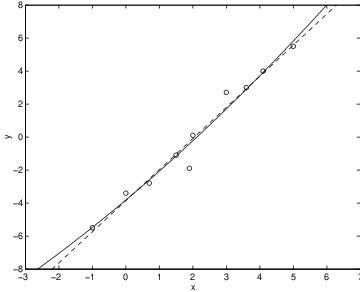
Suppose that we are given $n$ data points $(x_i,y_i)$ for $i=1,\ldots ,10$ . For example, consider the ten points

$\begin{equation} \label{E:scatterdata} \begin{array}{ccccc} (2.0,0.1) & (3.0,2.7) & (1.5,-1.1) & (-1.0,-5.5) & (0.0,-3.4)\\ (3.6,3.0) & (0.7,-2.8) & (4.1,4.0) & (1.9,-1.9) & (5.0,5.5) \end{array} \end{matlabEquation} The ten points $(x_i,y_i)$ are plotted in Figure~\ref{F:linreg} using the commands \begin{verbatim} e10_3_1 plot(X,Y,'o') axis([-3,7,-8,8]) xlabel('x') ylabel('y') \end{verbatim} \begin{figure}[htb] \centerline{% \psfig{file=../figures/linreg.eps,width=2.5in}} \caption{Scatter plot of data in \protect\eqref{E:scatterdata}.} \label{F:linreg} \end{figure} Next, suppose that there is a linear relation between the $x_i$ and the $y_i$; that is, we assume that there are constants $b_1$ and $b_2$ (that do not depend on $i$) for which $y_i=b_1+b_2x_i$ for each $i$. But these points are just data; errors may have been made in their measurement. So we ask: Find $b_1^0$ and $b_2^0$ so that the error made in fitting the data to the line $y=b_1^0+b_2^0x$ is minimal, that is, the error that is made in that fit is less than or equal to the error made in fitting the data to the line $y=b_1+b_2x$ for any other choice of $b_1$ and $b_2$. We begin by discussing what that error actually is. Given constants $b_1$ and $b_2$ and given a data point $x_i$, the difference between the data value\index{data value} $y_i$ and the hypothesized value $b_1+b_2x_i$ is the error that is made at that data point. Next, we combine the errors made at all of the data points; a standard way to combine the errors is to use the Euclidean distance\index{distance!Euclidean} \[ E(b) = \left((y_1-(b_1+b_2x_1))^2+\cdots+(y_{10}-(b_1+b_2x_{10}))^2\right)^{\half}. \] Rewriting $E(b)$ in vector notation leads to an economy in notation and to a conceptual advantage. Let \[ X=(x_1,\ldots,x_{10})^t \quad Y=(y_1,\ldots,y_{10})^t \AND F_1=(1,1,\ldots,1) \] be vectors in $\R^{10}$. Then in coordinates \[ Y-(b_1F_1+b_2X) = \left(\begin{array}{c} y_1-(b_1+b_2x_1)\\ \vdots\\ y_{10}-(b_1+b_2x_{10})\end{array}\right). \] It follows that \[ E(b) = ||Y-(b_1F_1+b_2X)||. \] The problem of making a least squares fit is to minimize $E$ over all $b_1$ and $b_2$. To solve the minimization problem\index{minimization problem}, note that the vectors $b_1F_1+b_2X$ form a two dimensional subspace $W=\Span\{F_1,X\}\subset\R^{10}$ \index{span} (at least when $X$ is not a scalar multiple of $F_1$, which is almost always). Minimizing $E$ is identical to finding a vector $w_0=b_1^0F_1+b_2^0X\in W$ that is nearest to the vector $Y\in\R^{10}$. This is the least squares\index{least squares} question that we solved in the Section~\ref{S:LSA}. We can use \Matlab to compute the values of $b_1^0$ and $b_2^0$ that give the best linear approximation to $Y$. If we set the matrix $A=(F_1|X)$, then Theorem~\ref{T:nearestvector} implies that the values of $b_1^0$ and $b_2^0$ are obtained using \eqref{E:nearestvector}. In particular, type {\tt e10\_3\_1} to call the vectors {\tt X, Y, F1} into \Matlabp, and then type \begin{verbatim} A = [F1 X]; b0 = inv(A'*A)*A'*Y \end{verbatim} to obtain \begin{verbatim} b0(1) = -3.8597 b0(2) = 1.8845 \end{verbatim} Superimposing the line $y=-3.8597+1.8845x$ on the scatter plot\index{scatter plot} in Figure~\ref{F:linreg} yields the plot in Figure~\ref{F:linreg2}. The total error is $E(b0)=1.9634$ (obtained in \Matlab by typing {\tt norm(Y-(b0(1)*F1+b0(2)*X)})\index{\computer!norm}. Compare this with the error $E(2,-4)=2.0928$. \begin{figure}[htb] \centerline{% \psfig{file=../figures/linreg2.eps,width=2.5in}} \caption{Scatter plot of data in \protect\eqref{E:scatterdata} with best linear approximation.} \label{F:linreg2} \end{figure} \subsubsection*{General Linear Regression} \index{linear!regression} We can summarize the previous discussion, as follows. Given $n$ data points \[ (x_1,y_1),\ldots, (x_n,y_n); \] form the vectors \[ X=(x_1,\ldots,x_n)^t \quad Y=(y_1,\ldots,y_n)^t \AND F_1=(1,\ldots,1)^t \] in $\R^n$. Find constants $b_1^0$ and $b_2^0$ so that $b_1^0F_1+b_2^0X$ is a vector in $W=\Span\{F_1,X\}\subset\R^n$ that is nearest to $Y$. Let \[ A=(F_1|X) \] be the $n\times 2$ matrix. This problem is solved by least squares in \eqref{E:nearestvector} as \begin{equation} \label{E:LSlinfit} \vectwo{b_1^0}{b_2^0} = (A^tA)\inv A^tY. \end{equation}$

Least Squares Fit to a Quadratic Polynomial

Suppose that we want to fit the data $(x_i,y_i)$ to a quadratic polynomial $y=b_1+b_2x+b_3x^2$ by least squares methods. We want to find constants $b_1^0,b_2^0,b_3^0$ so that the error made is using the quadratic polynomial $y=b_1^0+b_2^0x+b_3^0x^2$ is minimal among all possible choices of quadratic polynomials. The least squares error is $E(b) = ||Y-\left (b_1F_1+b_2X+b_3X^{(2)}\right )||$ where $X^{(2)}=\left (x_1^2,\ldots ,x_n^2\right )^t$ and, as before, $F_1$ is the $n$ vector with all components equal to $1$ .

We solve the minimization problem as before. In this case, the space of possible approximations to the data $W$ is three dimensional; indeed, $W=\Span \{F_1,X,X^{(2)}\}$ . As in the case of fits to lines we try to find a point in $W$ that is nearest to the vector $Y\in \R ^n$ . By (??), the answer is: $b = (A^tA)\inv A^tY,$ where $A=(F_1|X|X^{(2)})$ is an $n\times 3$ matrix.

Suppose that we try to fit the data in (??) with a quadratic polynomial rather than a linear one. Use MATLAB as follows

e10_3_1
 
A = [F1 X X.*X];
 
b = inv(A’*A)*A’*Y;

to obtain

b0(1) =   0.0443
 
b0(2) =   1.7054
 
b0(3) =  -3.8197

So the best parabolic fit to this data is $y=-3.8197+1.7054x+0.0443x^2$ . Note that the coefficient of $x^2$ is small suggesting that the data was well fit by a straight line. Note also that the error is $E(b0)=1.9098$ which is only marginally smaller than the error for the best linear fit. For comparison, in Figure ?? we superimpose the equation for the quadratic fit onto Figure ??.

Figure 1: Scatter plot of data in (??) with best linear and quadratic approximations. The best linear fit is plotted with a dashed line.

General Least Squares Fit

The approximation to a quadratic polynomial shows that least squares fits can be made to any finite dimensional function space. More precisely, Let $\cal C$ be a finite dimensional space of functions and let $f_1(x),\ldots ,f_m(x)$ be a basis for $\cal C$ . We have just considered two such spaces: ${\cal C}=\Span \{f_1(x)=1,f_2(x)=x\}$ for linear regression and ${\cal C}=\Span \{f_1(x)=1,f_2(x)=x,f_3(x)=x^2\}$ for least squares fit to a quadratic polynomial.

The general least squares fit of a data set $(x_1,y_1),\ldots , (x_n,y_n)$ is the function $g_0(x)\in {\cal C}$ that is nearest to the data set in the following sense. Let $X = (x_1,\ldots ,x_n)^t \AND Y = (y_1,\ldots ,y_n)^t$ be column vectors in $\R ^n$ . For any function $g(x)$ define the column vector $G = (g(x_1),\ldots ,g(x_n))^t\in \R ^n.$ So $G$ is the evaluation of $g(x)$ on the data set. Then the error $E(g) = ||Y-G||$ is minimal for $g=g_0$ .

More precisely, we think of the data $Y$ as representing the (approximate) evaluation of a function on the $x_i$ . Then we try to find a function $g_0\in {\cal C}$ whose values on the $x_i$ are as near as possible to the vector $Y$ . This is just a least squares problem. Let $W\subset \R ^n$ be the vector subspace spanned by the evaluations of function $g\in {\cal C}$ on the data points $x_i$ , that is, the vectors $G$ . The minimization problem is to find a vector in $W$ that is nearest to $Y$ . This can be solved in general using (??). That is, let $A$ be the $n\times m$ matrix $A = (F_1|\cdots |F_m)$ where $F_j\in \R ^n$ is the column vector associated to the $j^{th}$ basis element of $\cal C$ , that is, $F_j = (f_j(x_1),\ldots ,f_j(x_n))^t\in \R ^n.$ The minimizing function $g_0(x)\in {\cal C}$ is a linear combination of the basis functions $f_1(x),\ldots ,f_n(x)$ , that is, $g_0(x) = b_1f_1(x) + \cdots + b_mf_m(x)$ for scalars $b_i$ . If we set $b = (b_1,\ldots ,b_m)\in \R ^m,$ then least squares minimization states that

$\begin{equation} \label{E:LSFG} b = (A'A)\inv A'Y. \end{equation}$

This equation can be solved easily in MATLAB. Enter the data as column $n$ -vectors X and Y. Compute the column vectors Fj = $f_j$ (X) and then form the matrix A = [F1 F2 $\cdots$ Fm]. Finally compute

b = inv(A’*A)*A’*Y

Least Squares Fit to a Sinusoidal Function

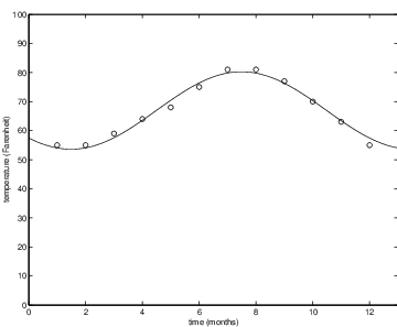
We discuss a specific example of the general least squares formulation by considering the weather. It is reasonable to expect monthly data on the weather to vary periodically in time with a period of one year. In Table ?? we give average daily high and low temperatures for each month of the year for Paris and Rio de Janeiro. We attempt to fit this data with curves of the form: $g(T) = b_1 + b_2\cos \left (\frac {2\pi }{12}T\right ) + b_3\sin \left (\frac {2\pi }{12}T\right ),$ where $T$ is time measured in months and $b_1,b_2,b_3$ are scalars. These functions are $12$ periodic, which seems appropriate for weather data, and form a three dimensional function space $\cal C$ . Recall the trigonometric identity $a\cos (\omega t) + c\sin (\omega t) = d\sin (\omega (t-\varphi ))$ where $d = \sqrt {a^2+c^2}.$ Based on this identity we call $\cal C$ the space of sinusoidal functions. The number $d$ is called the amplitude of the sinusoidal function $g(T)$ .


	Paris		Rio de Janeiro			Paris		Rio de Janeiro
Month	High	Low	High	Low	Month	High	Low	High	Low

1	55	39	84	73	7	81	64	75	63
2	55	41	85	73	8	81	64	76	64
3	59	45	83	72	9	77	61	75	65
4	64	46	80	69	10	70	54	77	66
5	68	55	77	66	11	63	46	79	68
6	75	61	76	64	12	55	41	82	71

Table 1: Monthly Average of Daily High and Low Temperatures in Paris and Rio de Janeiro.

Note that each data set consists of twelve entries — one for each month. Let $T=(1,2,\ldots ,12)^t$ be the vector $X\in \R ^{12}$ in the general presentation. Next let $Y$ be the data in one of the data sets — say the high temperatures in Paris.

Now we turn to the vectors representing basis functions in $\cal C$ . Let

F1=[1 1 1 1 1 1 1 1 1 1 1 1]’

be the vector associated with the basis function $f_1(T)=1$ . Let F2 and F3 be the column vectors associated to the basis functions $f_2(T) = \cos \left (\frac {2\pi }{12} T\right ) \AND f_3(T) = \sin \left (\frac {2\pi }{12} T\right ).$ These vectors are computed by typing

F2 = cos(2*pi/12*T);
 
F3 = sin(2*pi/12*T);

By typing temper, we enter the temperatures and the vectors T, F1, F2 and F3 into MATLAB.

To find the best fit to the data by a sinusoidal function $g(T)$ , we use (??). Let $A$ be the $12\times 3$ matrix

A = [F1 F2 F3];

The table data is entered in column vectors ParisH and ParisL for the high and low Paris temperatures and RioH and RioL for the high and low Rio de Janeiro temperatures. We can find the best least squares fit of the Paris high temperatures by a sinusoidal function $g_0(T)$ by typing

b = inv(A’*A)*A’*ParisH

obtaining

                                                                  

                                                                  
b(1) =  66.9167
 
b(2) =  -9.4745
 
b(3) =  -9.3688

The result is plotted in Figure ?? by typing

plot(T,ParisH,’o’)
 
axis([0,13,0,100])
 
xlabel(’time (months)’)
 
ylabel(’temperature (Fahrenheit)’)
 
hold on
 
xx = linspace(0,13);
 
yy = b(1) + b(2)*cos(2*pi*xx/12) +
 
     b(3)*sin(2*pi*xx/12);
 
plot(xx,yy)

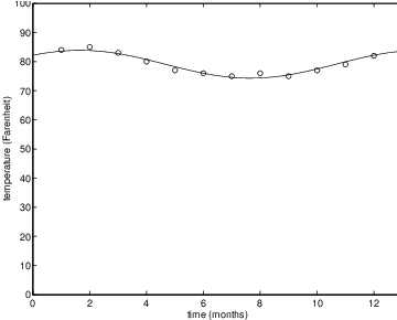
Figure 2: Monthly averages of daily high temperatures in Paris (left) and Rio de Janeiro (right) with best sinusoidal approximation.

A similar exercise allows us to compute the best approximation to the Rio de Janeiro high temperatures obtaining

b(1) =  79.0833
 
b(2) =   3.0877
 
b(3) =   3.6487

The value of $b(1)$ is just the mean high temperature and not surprisingly that value is much higher in Rio than in Paris. There is yet more information contained in these approximations. For the high temperatures in Paris and Rio $d_P = 13.3244 \AND d_R = 4.7798.$ The amplitude $d$ measures the variation of the high temperature about its mean. It is much greater in Paris than in Rio, indicating that the difference in temperature between winter and summer is much greater in Paris than in Rio.

Least Squares Fit in MATLAB

The general formula for a least squares fit of data (??) has been preprogrammed in MATLAB. After setting up the matrix $A$ whose columns are the vectors $F_j$ just type

b = A\Y

This MATLAB command can be checked on the sinusoidal fit to the high temperature Rio de Janeiro data by typing

b = A\RioH

and obtaining

b =
   79.0833
    3.0877
    3.6487

Exercises

World population data for each decade of this century (except for 1910) is given in Table ??. Assume that population growth is linear $P=mT+b$ where time $T$ is measured in decades since the year 1900 and $P$ is measured in billions of people. This data can be recovered by typing e10_3_po.

Find $m$ and $b$ to give the best linear fit to this data.
Use this linear approximation to the data to make predictions of the world populations in the year 1910 and 2000.
Do you expect the prediction for the year 2000 to be high or low or on target? Explain why by graphing the data with the best linear fit superimposed and by using the differential equation population model discussed in Section ??.


Year	Population (in millions)	Year	Population (in millions)

1900	1625	1950	2516
1910	n.a.	1960	3020
1920	1813	1970	3698
1930	1987	1980	4448
1940	2213	1990	5292

Table 2: Twentieth Century World Population Data by Decades.

Find the best sinusoidal approximation to the monthly average low temperatures in Paris and Rio de Janeiro. How does the variation of these temperatures about the mean compare to the high temperature calculations? Was this the result you expected?

In Table ?? we present weather data from ten U.S. cities. The data is the average number of days in the year with precipitation and the percentage of sunny hours to hours when it could be sunny. Find the best linear fit to this data.


City	Rainy Days	Sunny (%)	City	Rainy Days	Sunny (%)

Charleston	92	72	Kansas City	98	59
Chicago	121	54	Miami	114	85
Dallas	82	65	New Orleans	103	61
Denver	82	67	Phoenix	28	88
Duluth	136	52	Salt Lake City	99	59

Table 3: Precipitation Days Versus Sunny Time for Selected U.S. Cities.