Algebraic operations such as addition and multiplication are performed on numbers while the calculus operations of differentiation and integration are performed on functions. Thus algebraic equations (such as ) are solved for numbers () while differential (and integral) equations are solved for functions.
In Chapter ?? we discussed how to solve systems of linear equations, such as
Solving a single linear equation in one unknown is a simple task. For example, solve for . Solving a single differential equation in one unknown function is far from trivial.
Integral Calculus as a Differential Equation
Mathematically, the simplest type of differential equation is:
where is some continuous function. In words, this equation asks us to find all functions whose derivative is . The fundamental theorem of calculus tells us the answer: is an antiderivative of . Thus to find all solutions, we just integrate both sides of (??) with respect to . Formally, using indefinite integrals, where is an arbitrary constant. (It is tempting to put a constant of integration on both sides of (??), but two constants are not needed, as we can just combine both constants on the right hand side of this equation.) Since the indefinite integral of is just the function , we have In particular, finding closed form solutions to differential equations of the type (??) is equivalent to finding all definite integrals of the function . Indeed, to find closed form solutions to differential equations like (??) we need to know all of the techniques of integration from integral calculus.Initial Conditions and the Role of the Integration Constant
Equation (??) tells us that there are an infinite number of solutions to the differential equation (??), each one corresponding to a different choice of the constant . To understand how to interpret the constant , consider the example Using (??) we see that the answer is Note that Thus, the constant represents an initial condition for the differential equation. We will return to the discussion of initial conditions several times in this chapter.
See Exercise ?? for a more interesting example of this type of differential equation.
Solutions to Differential Equations are Functions
Consider the differential equation
Are the functions solutions to the differential equation (??)?To test whether or not the function is a solution, we compute the left and right hand sides of (??):
To test whether or not the function is a solution, we again compute the left and right hand sides of (??):
Note that we have not discussed how we knew that the function is a solution to (??). For the most part, the issue of how one finds solutions to a differential equation will be discussed in later chapters, though we do determine solutions to a very important equation next.
The Linear Differential Equation of Growth and Decay
The real subject of differential equations begins when the function on the right hand side of (??) depends explicitly on the function , and the simplest such differential equation is: Using results from calculus, we can solve this equation; indeed, we can solve the slightly more complicated equation
where is a constant. The differential equation (??) is linear since appears by itself on the right hand side. Moreover, (??) is homogeneous since the constant function is a solution.In words (??) asks: For which functions is the derivative of a scalar multiple of . The function is such a function, since More generally, the function
is a solution to (??) for any real constant . We claim that the functions (??) list all (differentiable) functions that solve (??).To verify this claim, we let be a solution to (??) and show that the ratio is a constant (independent of ). Using the product rule and (??), compute
Next, we discuss the role of the constant . We have written the function as , and we have meant the reader to think of the variable as time. Thus is the initial value of the function at time ; we say that is the initial value of . From (??) we see that and that is the initial value of the solution of (??). Henceforth, we write as so that the notation calls attention to the special meaning of this constant.
By deriving (??) we have proved:
As a consequence of Theorem ?? we see that there is a qualitative difference in the behavior of solutions to (??) depending on whether or . Suppose that . Then
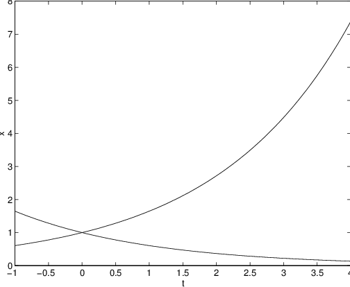
When we say that the solution has exponential growth and when we say that the solution has exponential decay . In either case, however, the number is called the growth rate. We can visualize this discussion by graphing the solutions in MATLAB.Suppose we set and . Type
x0 = 1;The result of this calculation is shown in Figure ??. In this way we can actually see the difference between exponential growth () and exponential decay (), as discussed in (??).
lambda = 0.5;
t = linspace(-1,4,100);
x = x0*exp(lambda*t);
plot(t,x)
hold on
xlabel(’t’)
ylabel(’x’)
lambda = -0.5;
x = x0*exp(lambda*t);
plot(t,x)
The Inhomogeneous Linear Differential Equation
It follows from (??) that solutions to the linear homogeneous differential equation (??) are either unbounded as or they approach zero. Now we consider an inhomogeneous differential equation and show that solutions can approach fixed values for increasing that are neither zero nor infinity.
As an example, consider the linear differential equation
Observe that is not a solution of (??) and therefore that (??) is inhomogeneous. It is easy to verify, however, that the constant function is a solution.Equation (??) can be solved by introducing a new function that transforms (??) into a homogeneous equation. Let and compute
Using Theorem ??, it follows that has the form Therefore is a solution of (??) for every constant . Moreover, which is neither zero nor infinity.
Any equation of the form
can be solved in a similar fashion. Just set It follows from (??) that Theorem ?? implies that for some constant and Note that the limit of as is when .Some Examples of (??)
Even though the differential equation (??) is one of the simplest differential equations, it still has some use in applications. We present two here: compound interest and population dynamics.
Compound Interest
Banks pay interest on an account in the following way. At the end of each day, the bank determines the interest rate for that day, checks the principal in the account, and then deposits an additional . So the next day the principal in this account is . Note that if denotes the interest rate per year, then . Of course, a day is just a convenient measure for elapsed time. Before computers were prevalent, banks paid interest yearly or quarterly or monthly or, in a few cases, even weekly, depending on the particular bank rules.
Observe that the more frequently interest is paid, the more money is earned. For example, if interest is paid only once at the end of a year, then the money in the account at the end of the year is , and the amount is called simple interest. But if interest is paid twice a year, then the principal at the end of six months will be , and the principal at the end of the year will be . Since there is more money in the account at the end of the year if the interest is compounded semiannually rather than annually. But how much is the difference and what is the maximum earning potential?
While making the calculation in the previous paragraph, we implicitly made a number of simplifying assumptions. In particular, we assumed
- an initial principal is deposited in the bank on January 1,
- the money is not withdrawn for one year,
- no new money is deposited in that account during the year,
- the yearly interest rate remains constant throughout the year, and
- interest is added to the account times during the year.
In this model, simple interest corresponds to , compound monthly interest to , and compound daily interest to .
We first answer the question: How much money is in this account after one year? After one time unit of year, the amount of money in the account is The interest rate in each time period is , the yearly rate divided by the number of time periods . Here we have used the assumption that the interest rate remains constant throughout the year. After two time units, the principal is: and at the end of the year (that is, after time periods)
Here we have used the assumption that money is neither deposited nor withdrawn from our account. Note that is the amount of money in the bank after one year assuming that interest has been compounded (equally spaced) times during that year, and the effective interest rate when compounding times is:For the curious, we can write a program in MATLAB to compute (??). Suppose we assume that the initial deposit , the simple interest rate is per year, and the interest payments are made monthly. In MATLAB type
N  = 12;

P0 = 1000;

r  = 0.06;

QN = (1 + r/N)^N*P0
The answer is , and the effective interest rate for monthly payments is . For
daily interest payments , the answer is , and the effective interest rate is
.
To find the maximum effective interest, we ask the bank to compound interest continuously; that is, we ask the bank to compute We compute this limit using differential equations. The concept of continuous interest is rephrased as follows. Let be the principal at time , where is measured in units of years. Suppose that we assume that interest is compounded times during the year. The length of time in each compounding period is and the change in principal during that time period is It follows that and, on taking the limit , we have the differential equation
Since the solution of the initial value problem given in Theorem ?? shows that After one year () we find that Note that and we have thus verified that Thus the maximum effective interest rate is . When the maximum effective interest rate is .
An Example from Population Dynamics
To provide a second interpretation of the constant in (??), we discuss a simplified model for population dynamics. Let be the size of a population of a certain species at time and let be the rate at which the population is changing at time . In general, depends on the time and is a complicated function of birth and death rates and of immigration and emigration, as well as of other factors. Indeed, the rate may well depend on the size of the population itself. (Overcrowding can be modeled by assuming that the death rate increases with the size of the population.) These population models assume that the rate of change in the size of the population is given by
they just differ on the precise form of . In general, the rate will depend on the size of the population as well as the time , that is, is a function .The simplest population model — which we now assume — is the one in which is assumed to be constant. Then equation (??) is identical to (??) after identifying with and with . Hence we may interpret as the growth rate for the population. The form of the solution in (??) shows that the size of a population grows exponentially if and decays exponentially if .
The mathematical description of this simplest population model shows that the assumption of a constant growth rate leads to exponential growth (or exponential decay). Is this realistic? Surely, no population will grow exponentially for all time, and other factors, such as limited living space, have to be taken into account. On the other hand, exponential growth describes well the growth in human population during much of human history. So this model, though surely oversimplified, gives some insight into population growth.
Exercises
In Exercises ?? – ?? find solutions to the given initial value problems.
In Exercises ?? – ?? determine whether or not each of the given functions and is a solution to the given differential equation.
One day it started snowing at a steady rate. A snowplow started at noon and went two miles in the first hour and one mile in the second hour. Assume that the speed of the snowplow times the depth of the snow is constant. At what time did it start to snow?
To set up this problem, let be the depth of the snow at time where is measured in hours and is noon. Since the snow is falling at a constant rate , where is the time that it started snowing. Let be the position of the snowplow along the road. The assumption that speed times the depth equals a constant means that where . The information about how far the snowplow goes in the first two hours translates to Now solve the problem.
In Exercises ?? – ?? use MATLAB to graph the given function on the specified interval.
Hint: Use the fact that the trigonometric functions and can be evaluated in MATLAB in the same way as the exponential function, that is, by using sin and cos instead of exp.