Phase Space Pictures and Equilibria

$\newenvironment {prompt}{}{} \newcommand {\Sec }[2]{\section {#1}} \newcommand {\trademark }[0]{{R\!\!\!\!\!\bigcirc }} \newcommand {\EXER }[0]{\section *{Exercises}} \newcommand {\CEXER }[0]{} \newcommand {\TEXER }[0]{} \newcommand {\R }[0]{\mbox {$\Bbb {R}$}} \newcommand {\C }[0]{\mbox {$\Bbb {C}$}} \newcommand {\Z }[0]{\mbox {$\Bbb {Z}$}} \newcommand {\N }[0]{\mbox {$\Bbb {N}$}} \newcommand {\D }[0]{\mbox {{\bf D}}} \newcommand {\setmin }[0]{\;\mbox {--}\;} \newcommand {\Matlab }[0]{{M\small {AT\-LAB}} } \newcommand {\Matlabp }[0]{{M\small {AT\-LAB}}} \newcommand {\computer }[0]{\Matlab Instructions} \newcommand {\half }[0]{\mbox {$\frac {1}{2}$}} \newcommand {\compose }[0]{\raisebox {.15ex}{\mbox {{\scriptsize $\circ $}}}} \newcommand {\AND }[0]{\quad \mbox {and}\quad } \newcommand {\vect }[2]{\left (\begin {array}{c} #1_1 \\ \vdots \\ #1_{#2}\end {array}\right )} \newcommand {\mattwo }[4]{\left (\begin {array}{rr} #1 & #2\\ #3 &#4\end {array}\right )} \newcommand {\mattwoc }[4]{\left (\begin {array}{cc} #1 & #2\\ #3 &#4\end {array}\right )} \newcommand {\vectwo }[2]{\left (\begin {array}{r} #1 \\ #2\end {array}\right )} \newcommand {\vectwoc }[2]{\left (\begin {array}{c} #1 \\ #2\end {array}\right )} \newcommand {\inv }[0]{^{-1}} \newcommand {\CC }[0]{{\cal C}} \newcommand {\CCone }[0]{\CC ^1} \newcommand {\Span }[0]{{\rm span}} \newcommand {\rank }[0]{{\rm rank}} \newcommand {\trace }[0]{{\rm tr}} \newcommand {\RE }[0]{{\rm Re}} \newcommand {\IM }[0]{{\rm Im}} \newcommand {\nulls }[0]{{\rm null\;space}} \newcommand {\dps }[0]{\displaystyle } \newcommand {\arraystart }[0]{\renewcommand {\arraystretch }{1.8}} \newcommand {\arrayfinish }[0]{\renewcommand {\arraystretch }{1.2}} \newcommand {\Start }[1]{\vspace {0.08in}\noindent {\bf Section~\ref {#1}}} \newcommand {\exer }[1]{\noindent {\bf \ref {#1}}} \newcommand {\ans }[0]{} \newcommand {\matthree }[9]{\left (\begin {array}{rrr} #1 & #2 & #3 \\ #4 & #5 & #6 \\ #7 & #8 & #9\end {array}\right )} \newcommand {\cvectwo }[2]{\left (\begin {array}{c} #1 \\ #2\end {array}\right )} \newcommand {\cmatthree }[9]{\left (\begin {array}{ccc} #1 & #2 & #3 \\ #4 & #5 & #6 \\ #7 & #8 & #9\end {array}\right )} \newcommand {\vecthree }[3]{\left (\begin {array}{r} #1 \\ #2 \\ #3\end {array}\right )} \newcommand {\cvecthree }[3]{\left (\begin {array}{c} #1 \\ #2 \\ #3\end {array}\right )} \newcommand {\cmattwo }[4]{\left (\begin {array}{cc} #1 & #2\\ #3 &#4\end {array}\right )} \newcommand {\thehelp }[0]{\thesection .\arabic {equation}} \newcommand {\matlabEquation }[0]{\let \oldtheequation \theequation \renewcommand {\theequation }{\oldtheequation *}\begin {equation}} \newcommand {\HyperFirstAtBeginDocument }[0]{\AtBeginDocument } \newcommand {\epstopdfsetup }[0]{\setkeys {ETE}} changed the theorem header of amsthm failed\MessageBreak }}} \newcommand {\GetTitleStringSetup }[0]{\setkeys {gettitlestring}} \newcommand {\Sectionformat }[2]{#1}$ $% This file was *autogenerated* from phaseSpacePicturesAndEquilibria.sagetex.sage with % sagetex.py version 2015/08/26 v3.0-92d9f7a %368a6c6ac14741e248f6f10bbe8a9515% md5sum of corresponding .sage file (minus "goboom","current_tex_line",and pause/unpause lines)$

Recall that in a phase space plot, the solution $x(t)$ represents the position $x$ of a particle on a line for each time $t$ . Phase space plots are difficult to draw, since motion must be built into the plot. However, we can view this dynamically in MATLAB using the program pline.

In this discussion, we will only plot solutions of autonomous, first order differential equations; that is, equations of the form $\dot {x} = g(x).$ To begin, type

pline

and the window with the PLINE Setup appears on the computer screen. The layout is essentially the same as in the DFIELD5 Setup described above. However, there are two differences:

(a): Since we assume that our equation is autonomous, the time variable — the independent variable — does not appear explicitly and no time interval is specified. Rather the Integration time, the period for which the solution is to be computed, has to be declared. This change is due to the convention that all numerical computations start at $t=0$ .
(b): We may enter equations with one free parameter. In the PLINE Setup that parameter is lambda. Moreover, we may choose the value for that parameter. The default value in the PLINE Setup is $-0.8$ . Hence, the default equation used by pline is equation (??) with $\lambda = -0.8$ .

When we click with the left mouse button onto the button Proceed, then the display window with the title PLINE Display opens and the $x$ -axis shown in Figure ?? becomes visible.

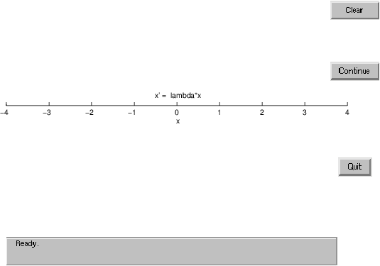
Figure 1: PLINE Display for $\dot {x}=\lambda x$ and $x\in [-4,4]$ .

Similar to dfield5 we may start the numerical solution by clicking with the left mouse button on the initial value of $x$ . It is not necessary to hit the axis precisely. For example, when we click (approximately) on $3$ , a colored disk becomes visible and moves to the left until it stops at a value for $x$ that is between $0.05$ and $0.06$ . This value can be read at the bottom of the window from the message Endpoint: 0.05…. We can also enter the initial point by choosing the option Keyboard input from the PLINE Options menu. In fact, if we enter $x=3$ in that window and click on Compute, then the corresponding solution is computed and we obtain the message Endpoint: 0.05495. Sometimes it helps to clear all markers in the display window; this is accomplished by clicking on Clear.

Equilibria and Dynamics

The simplest solution to a differential equation is a solution that remains constant for all time. Such solutions are called equilibria. Equilibria are found as follows:

Consider the autonomous differential equation $\begin{equation} \label{aut} \frac{dx}{dt}(t) = g(x(t)). \end{equation}$ Then $x(t)=x_0$ is an equilibrium if and only if $g(x_0)=0$ .

Proof: Suppose that $x(t)=x_0$ is an equilibrium solution to (??). Then $g(x_0)=0$ , since $dx/dt = 0$ . Conversely, suppose $g(x_0)=0$ . Then $x(t)=x_0$ is a solution to (??). $\blacksquare$

We now return to pline and the autonomous equation $g(x)=-0.8x$ . If we continue the integration by pushing Continue in the display window we see again that the solution approaches $0$ as $t$ goes to infinity; that is, the solution approaches the equilibrium given by $x(t)=0$ . Correspondingly, the point that indicates the position of $x(t)$ in the display window does not move any more. Solutions that have initial conditions near $0$ either tend towards $0$ when $\lambda < 0$ or away from $0$ when $\lambda > 0$ .

An equilibrium $x(t)=x_0$ is asymptotically stable if all solutions $y(t)$ with initial condition $y(0)$ near $x_0$ have the limit $x_0$ as $t$ goes to infinity. In symbols we require $\lim _{t\to \infty } y(t) = x_0.$ (The definition of asymptotic stability is more complicated in higher dimensions.) The equilibrium $x(t)=x_0$ is unstable if trajectories starting near $x_0$ move away from $x_0$ . Thus, in our example, the equilibrium $x=0$ is asymptotically stable when $\lambda < 0$ and unstable when $\lambda > 0$ .

The dynamical behavior of autonomous differential equations of the form (??) is essentially determined by the equilibria of $g$ . We explore this statement by using pline to analyze the dynamical behavior of the ordinary differential equation

$\begin{equation} \label{pitch_eq} \dot{x} = x(\lambda-x^2), \end{equation}$ where $\lambda$ is a constant.

First, enter this equation by editing the upper box in the PLINE Setup window. Do this editing by clicking in the window and deleting the default equation and then type x*(lambda-x2). Then change the minimum and maximum values of $x$ from $-4$ and $4$ to $-2$ and $2$ . Finally, change the integration time to $1$ and the value of lambda to $-1$ .

Second, push on Proceed so that the $x$ axis becomes visible in the display window. On integrating the system, we find that solutions seem to behave in a similar way to the solutions of (??) for $\lambda < 0$ : all the solutions approach zero as $t$ goes to infinity. Indeed, we can see that $x(t)=0$ is an equilibrium solution of (??) for all values of $\lambda$ . When $\lambda <0$ numerical exploration suggests that $0$ is an asymptotically stable equilibrium.

We now explore the stability properties of $x(t)=0$ when $\lambda >0$ . We begin by changing the value of $\lambda$ to $+1$ . We do this in the setup window and afterwards we confirm the change by pushing Proceed. If we now compute solutions of the differential equation, then we see that they come to a rest at $+1$ if we start with a positive value for $x(0)$ whereas they approach $-1$ if we start with a negative value for $x(0)$ . Even if we begin the numerical computation very close to $x=0$ , the solutions tend to either $+1$ or $-1$ . These calculations indicate that $0$ is an unstable equilibrium while both $+1$ and $-1$ are stable equilibria of (??) when $\lambda =1$ .

We use the Keyboard input to check that $x(t) = +1$ or $x(t) = -1$ are equilibrium solutions. Start the computations with initial values $x(0) = +1$ or $x(0) = -1$ and see that the solutions remain constant in time. Alternatively, solve the equation $x(1-x^2) = 0,$ to see that $x=0,1,-1$ are all equilibria of (??) when $\lambda =1$ .

Our numerical computations indicate that changing the value of $\lambda$ from $-1$ to $+1$ changes the stability property of the equilibrium $x(t)=0$ .

We can now discuss a method for completely determining the dynamics of a single autonomous differential equation (??) — assuming that equilibria are isolated.

Determine all equilibria of (??) by solving the equation $g(x)=0$ .
Choose an initial point between each pair of consecutive equilibria and determine the direction of motion (sign of $g$ ) at that initial point. This can be done either directly or by using pline.
On a line plot the equilibria and connect them by arrows indicating the direction of the dynamics.

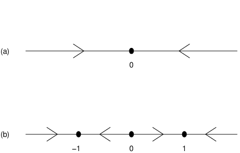
For example, the dynamics of the differential equations $\dot {x} = x(-1-x^2)$ and $\dot {x} = x(1-x^2)$ are shown schematically in Figure ??.

Figure 2: Schematic dynamics of (a) $\dot {x}=x(-1-x^2)$ and (b) $\dot {x}=x(1-x^2)$ .

Hyperbolic Equilibria

Suppose that $x_0$ is an equilibrium for (??); that is suppose $g(x_0)=0$ . We denote the derivative of $g(x)$ with respect to $x$ , $dg/dx$ , by $g'$ . The equilibrium $x_0$ is hyperbolic if $g'(x_0)\neq 0$ . Assume that $x_0$ is a hyperbolic equilibrium and use the tangent line approximation to $g(x)$ near $x_0$ ( $\Delta g = g'(x_0)\Delta x$ ) and that fact that $g(x_0)=0$ to conclude that $g(x) \approx g'(x_0)(x-x_0).$ It follows that if $g'(x_0)<0$ , then $g(x)$ is negative when $x>x_0$ and positive when $x<x_0$ . So when $g'(x_0)<0$ , solutions of (??) starting just to the right of $x_0$ will move left ( $g<0$ ) and tend towards $x_0$ and solutions starting just to the left of $x_0$ will move right ( $g>0$ ) and tend towards $x_0$ . Similarly, if $g'(x_0)>0$ , then $g(x)$ is positive when $x>x_0$ and negative when $x<x_0$ . Thus, solutions near $x_0$ will tend away from $x_0$ when $g'(x_0)>0$ . We have shown:

Stability of Hyperbolic Equilibria Let $x_0$ be a hyperbolic equilibrium for the differential equation $\frac {dx}{dt} = g(x).$ If $g'(x_0)<0$ , then the equilibrium is asymptotically stable; and if $g'(x_0)>0$ , then the equilibrium is unstable.

It follows from Theorem ?? that the phase line picture near a hyperbolic equilibrium is particularly simple as the arrows beside that equilibrium either both point towards the equilibrium (as in Figure ??(a)) or both point away from the equilibrium (as near $0$ in Figure ??(b)).

Comparing Phase Lines and Time Series

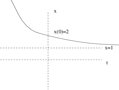
Phase line plots and time series graphs give different ways of presenting the same information. With that point in mind, it is important to be able to recreate one type of plot from the other. For example, let $x(t)$ be the solution to the differential equation $\dot {x}=x(1-x^2)$ with initial condition $x(0)=2$ . In Figure ??(b) we have drawn the schematic phase line for all solutions to this differential equation. How can we reconstruct a (schematic) graph of the time series $x(t)$ for this solution just from the phase line?

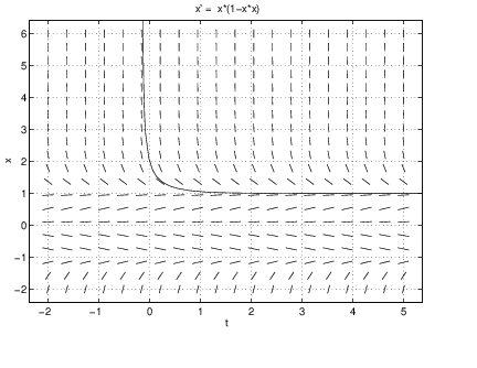
To answer this question, note that in Figure ??(b) the initial condition $x(0)=2$ lies to the right of all equilibria of this equation, and the arrow indicates that solution trajectories starting in this area move to the left, that is, they decrease to the equilibrium at $x=1$ . It follows that $\lim _{t\to \infty } x(t) = 1.$ Since there are no equilibria to the right of $x=2$ , the graph of $x(t)$ must increase to infinity in backwards time. So the graph of $x=x(t)$ is decreasing and asymptotic to $x=1$ for large positive $t$ . A schematic graph is given in Figure ??(a). Using dfield5 we can check this description by numerically integrating the differential equation. This graph is shown in Figure ??(b).

Figure 3: Time series for solution to $\dot {x}=x(1-x^2)$ with $x(0)=2$ . (Left) Sketch using asymptotic information; (right) dfield5 computation.

Exercises

Use pline to find an initial condition $x(0)$ for the ordinary differential equation (??) with $\lambda =-0.2$ such that the corresponding solution $x(t)$ satisfies $x(20)\in [0.001,0.002]$ .

Use pline to find all the equilibria of the ordinary differential equation $\dot {x} = (x^2-1)(x+2).$ Which of the equilibria are stable and which are unstable?

Consider the following ordinary differential equation: $\dot {x} = \lambda x(1-x).$ Use pline to find a value for the parameter $\lambda$ such that $x(t)=1$ is a stable equilibrium.

The differential equation $\frac {dx}{dt} = x^2$ has an equilibrium at the origin. Use pline to determine those $x_0$ for which solutions to the initial value $x(0)=x_0$ tend towards the origin.

Consider the differential equation $\frac {dx}{dt} = a x^3.$ Use pline to verify that the origin is an asymptotically stable equilibrium when $a = -1$ and is an unstable equilibrium when $a = +1$ . Discuss the relationship between these examples and Theorem ??.

In Exercises ?? – ?? compute the equilibria of the given differential equation, determine whether these equilibria are asymptotically stable or unstable, and draw a schematic of the dynamics of this equation like the one in Figure ??. You may use pline to check your answer.

$\dot {x} = x^2 + 2x - 3$ .

$\dot {x} = x^3 - 2x^2 - 8x$ .

$\dot {x} = x^3 + 2x^2 - 3x$ .

$\dot {x} = x^2 + 6x + 1$ .

Let $x(t)$ be a solution to the initial value problem

$\begin{eqnarray*} \dot{x} & = & g(x) \\ x(0) & = & x_0. \end{eqnarray*}$

Let $y(t)=x(-t)$ . Show that $y(t)$ is a solution to the initial value problem

$\begin{eqnarray*} \dot{y} & = & -g(y) \\ y(0) & = & x_0. \end{eqnarray*}$

(Thus, to integrate the solution $x(t)$ backwards in time is the same as solving the differential equation $\dot {y} = -g(y)$ forward in time.)

Use Exercise ?? to devise a shortcut for solving Exercise ??.

Sketch the time series for the solution to the differential equation pictured in Figure ??(b) with initial condition $x(0)=\frac {1}{2}$ . Use only the phase space plot given in this figure. Use dfield5 to verify your answer.

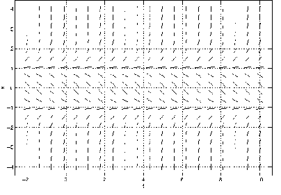
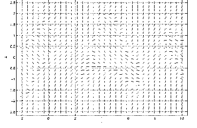
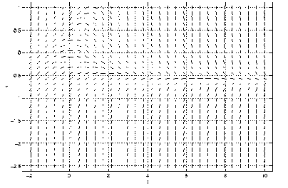
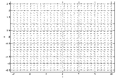
In Exercises ?? – ?? use the line field given in Figure ?? to answer the following:
(a) Is the differential equation that was used to draw this figure autonomous or nonautonomous.
(b) If the differential equation is autonomous, then draw the phase line noting the values of $x$ where equilibria occur and whether they are asymptotically stable or not. If the differential equation is nonautonomous, then draw the time series for solutions with initial conditions $x(0)=0$ and $x(2)=0$ .

Use Figure ??(i) to answer parts (a) and (b).

Use Figure ??(ii) to answer parts (a) and (b).

Use Figure ??(iii) to answer parts (a) and (b).

Use Figure ??(iv) to answer parts (a) and (b).

(i) (ii)

(iii) (iv)

Figure 4: Figures for Exercises ?? – ??