The Geometry of Low-Dimensional Solutions

$\newenvironment {prompt}{}{} \newcommand {\Sec }[2]{\section {#1}} \newcommand {\trademark }[0]{{R\!\!\!\!\!\bigcirc }} \newcommand {\EXER }[0]{\section *{Exercises}} \newcommand {\CEXER }[0]{} \newcommand {\TEXER }[0]{} \newcommand {\R }[0]{\mbox {$\Bbb {R}$}} \newcommand {\C }[0]{\mbox {$\Bbb {C}$}} \newcommand {\Z }[0]{\mbox {$\Bbb {Z}$}} \newcommand {\N }[0]{\mbox {$\Bbb {N}$}} \newcommand {\D }[0]{\mbox {{\bf D}}} \newcommand {\setmin }[0]{\;\mbox {--}\;} \newcommand {\Matlab }[0]{{M\small {AT\-LAB}} } \newcommand {\Matlabp }[0]{{M\small {AT\-LAB}}} \newcommand {\computer }[0]{\Matlab Instructions} \newcommand {\half }[0]{\mbox {$\frac {1}{2}$}} \newcommand {\compose }[0]{\raisebox {.15ex}{\mbox {{\scriptsize $\circ $}}}} \newcommand {\AND }[0]{\quad \mbox {and}\quad } \newcommand {\vect }[2]{\left (\begin {array}{c} #1_1 \\ \vdots \\ #1_{#2}\end {array}\right )} \newcommand {\mattwo }[4]{\left (\begin {array}{rr} #1 & #2\\ #3 &#4\end {array}\right )} \newcommand {\mattwoc }[4]{\left (\begin {array}{cc} #1 & #2\\ #3 &#4\end {array}\right )} \newcommand {\vectwo }[2]{\left (\begin {array}{r} #1 \\ #2\end {array}\right )} \newcommand {\vectwoc }[2]{\left (\begin {array}{c} #1 \\ #2\end {array}\right )} \newcommand {\inv }[0]{^{-1}} \newcommand {\CC }[0]{{\cal C}} \newcommand {\CCone }[0]{\CC ^1} \newcommand {\Span }[0]{{\rm span}} \newcommand {\rank }[0]{{\rm rank}} \newcommand {\trace }[0]{{\rm tr}} \newcommand {\RE }[0]{{\rm Re}} \newcommand {\IM }[0]{{\rm Im}} \newcommand {\nulls }[0]{{\rm null\;space}} \newcommand {\dps }[0]{\displaystyle } \newcommand {\arraystart }[0]{\renewcommand {\arraystretch }{1.8}} \newcommand {\arrayfinish }[0]{\renewcommand {\arraystretch }{1.2}} \newcommand {\Start }[1]{\vspace {0.08in}\noindent {\bf Section~\ref {#1}}} \newcommand {\exer }[1]{\noindent {\bf \ref {#1}}} \newcommand {\ans }[0]{} \newcommand {\matthree }[9]{\left (\begin {array}{rrr} #1 & #2 & #3 \\ #4 & #5 & #6 \\ #7 & #8 & #9\end {array}\right )} \newcommand {\cvectwo }[2]{\left (\begin {array}{c} #1 \\ #2\end {array}\right )} \newcommand {\cmatthree }[9]{\left (\begin {array}{ccc} #1 & #2 & #3 \\ #4 & #5 & #6 \\ #7 & #8 & #9\end {array}\right )} \newcommand {\vecthree }[3]{\left (\begin {array}{r} #1 \\ #2 \\ #3\end {array}\right )} \newcommand {\cvecthree }[3]{\left (\begin {array}{c} #1 \\ #2 \\ #3\end {array}\right )} \newcommand {\cmattwo }[4]{\left (\begin {array}{cc} #1 & #2\\ #3 &#4\end {array}\right )} \newcommand {\thehelp }[0]{\thesection .\arabic {equation}} \newcommand {\matlabEquation }[0]{\let \oldtheequation \theequation \renewcommand {\theequation }{\oldtheequation *}\begin {equation}} \newcommand {\HyperFirstAtBeginDocument }[0]{\AtBeginDocument } \newcommand {\epstopdfsetup }[0]{\setkeys {ETE}} changed the theorem header of amsthm failed\MessageBreak }}} \newcommand {\GetTitleStringSetup }[0]{\setkeys {gettitlestring}} \newcommand {\Sectionformat }[2]{#1}$ $% This file was *autogenerated* from theGeometryOfLowDimensionalSolutions.sagetex.sage with % sagetex.py version 2015/08/26 v3.0-92d9f7a %a6737c54ca83691c655b71cdde3e2088% md5sum of corresponding .sage file (minus "goboom","current_tex_line",and pause/unpause lines)$

In this section we discuss how to use MATLAB graphics to solve systems of linear equations in two and three unknowns. We begin with two dimensions.

Linear Equations in Two Dimensions

The set of all solutions to the equation

$\begin{equation} \label{2x-y=6} 2x - y = 6 \end{equation}$ is a straight line in the $xy$ plane; this line has slope $2$ and $y$ -intercept equal to $-6$ . We can use MATLAB to plot the solutions to this equation — though some understanding of the way MATLAB works is needed.

The plot command in MATLAB plots a sequence of points in the plane, as follows. Let $X$ and $Y$ be $n$ vectors. Then

plot(X,Y)

will plot the points $(X(1),Y(1))$ , $(X(2),Y(2))$ , …, $(X(n),Y(n))$ in the $xy$ -plane.

To plot points on the line (??) we need to enter the $x$ -coordinates of the points we wish to plot. If we want to plot a hundred points, we would be facing a tedious task. MATLAB has a command to simplify this task. Typing

x = linspace(-5,5,100);

produces a vector $x$ with $100$ entries with the $1^{st}$ entry equal to $-5$ , the last entry equal to $5$ , and the remaining $98$ entries equally spaced between $-5$ and $5$ . MATLAB has another command that allows us to create a vector of points x. In this command we specify the distance between points rather than the number of points. That command is:

x = -5:0.1:5;

Producing x by either command is acceptable.

Typing

y = 2*x - 6;

produces a vector whose entries correspond to the $y$ -coordinates of points on the line (??). Then typing

plot(x,y)

produces the desired plot. It is useful to label the axes on this figure, which is accomplished by typing

xlabel(’x’)
 
ylabel(’y’)

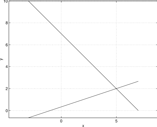
We can now use MATLAB to solve the equation (??) graphically. Recall that (??) is: $\arraycolsep 2pt \begin {array}{rcrcr} x & + & y & = & 7 \\ -x & + & 3y & = & 1 \end {array}$ A solution to this system of equations is a point that lies on both lines in the system. Suppose that we search for a solution to this system that has an $x$ -coordinate between $-3$ and $7$ . Then type the commands

x = linspace(-3,7,100);
 
y = 7 - x;
 
plot(x,y)
 
xlabel(’x’)
 
ylabel(’y’)
 
hold on
 
y = (1 + x)/3;
 
plot(x,y)
 
axis(’equal’)
 
grid

The MATLAB command hold on tells MATLAB to keep the present figure and to add the information that follows to that figure. The command axis(’equal’) instructs MATLAB to make unit distances on the $x$ and $y$ axes equal. The last MATLAB command superimposes grid lines. See Figure ??. From this figure you can see that the solution to this system is $(x,y)=(5,2)$ , which we already knew.

Figure 1: Graph of equations in (??)

There are several principles that follow from this exercise.

Solutions to a single linear equation in two variables form a straight line.
Solutions to two linear equations in two unknowns lie at the intersection of two straight lines in the plane.

It follows that the solution to two linear equations in two variables is a single point if the lines are not parallel. If these lines are parallel and unequal, then there are no solutions, as there are no points of intersection.

Linear Equations in Three Dimensions

We begin by observing that the set of all solutions to a linear equation in three variables forms a plane. More precisely, the solutions to the equation

$\begin{equation} \label{abcd} ax+by+cz=d \end{equation}$ form a plane that is perpendicular to the vector $(a,b,c)$ — assuming of course that the vector $(a,b,c)$ is nonzero.

This fact is most easily proved using the dot product. Recall from Chapter ?? (??) that the dot product is defined by $X\cdot Y = x_1y_1+x_2y_2+x_3y_3,$ where $X=(x_1,x_2,x_3)$ and $Y=(y_1,y_2,y_3)$ . We recall from Chapter ?? (??) the following important fact concerning dot products: $X\cdot Y = 0$ if and only if the vectors $X$ and $Y$ are perpendicular.

Suppose that $N=(a,b,c)\neq 0$ . Consider the plane that is perpendicular to the normal vector $N$ and that contains the point $X_0$ . If the point $X$ lies in that plane, then $X-X_0$ is perpendicular to $N$ ; that is,

$\begin{equation} \label{XX_0} (X-X_0)\cdot N = 0. \end{equation}$ If we use the notation $X=(x,y,z) \quad \mbox { and } \quad X_0=(x_0,y_0,z_0),$ then (??) becomes $a(x-x_0)+b(y-y_0)+c(z-z_0)=0.$ Setting $d=ax_0 + by_0 + cz_0$ puts equation (??) into the form (??). In this way we see that the set of solutions to a single linear equation in three variables forms a plane. See Figure ??.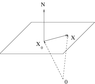

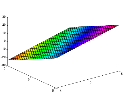
Figure 2: The plane containing $X_0$ and perpendicular to $N$ .

We now use MATLAB to visualize the planes that are solutions to linear equations. Plotting an equation in three dimensions in MATLAB follows a structure similar to the planar plots. Suppose that we wish to plot the solutions to the equation

$\begin{equation} \label{-2x+3y+z=2} -2x+3y+z=2. \end{equation}$ We can rewrite (??) as $z=2x-3y+2.$ It is this function that we actually graph by typing the commands

[x,y] = meshgrid(-5:0.5:5);
 
z = 2*x - 3*y + 2;
 
surf(x,y,z)

The first command tells MATLAB to create a square grid in the $xy$ -plane. Grid points are equally spaced between $-5$ and $5$ at intervals of $0.5$ on both the $x$ and $y$ axes. The second command tells MATLAB to compute the $z$ value of the solution to (??) at each grid point. The third command tells MATLAB to graph the surface containing the points $(x,y,z)$ . See Figure ??.

Figure 3: Graph of (??).

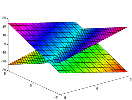
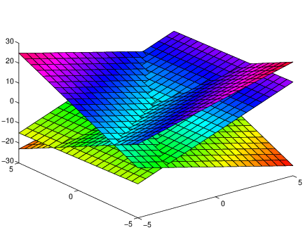
We can now see that solutions to a system of two linear equations in three unknowns consists of points that lie simultaneously on two planes. As long as the normal vectors to these planes are not parallel, the intersection of the two planes will be a line in three dimensions. Indeed, consider the equations

$\begin{eqnarray*} -2x + 3y + z & = & 2 \\ 2x - 3y + z & = & 0. \end{eqnarray*}$

We can graph the solution using MATLAB , as follows. We continue from the previous graph by typing

hold on
 
z = -2*x + 3*y;
 
surf(x,y,z)

The result, which illustrates that the intersection of two planes in $\R ^3$ is generally a line, is shown in Figure ??.

Figure 4: Line of intersection of two planes.

We can now see geometrically that the solution to three simultaneous linear equations in three unknowns will generally be a point — since generally three planes in three space intersect in a point. To visualize this intersection, as shown in Figure ??, we extend the previous system of equations to

$\begin{eqnarray*} -2x + 3y + z & = & 2 \\ 2x - 3y + z & = & 0\\ -3x + 0.2y + z & = & 1. \end{eqnarray*}$

Continuing in MATLAB type

z = 3*x - 0.2*y + 1;
 
surf(x,y,z)

Figure 5: Point of intersection of three planes.

Unfortunately, visualizing the point of intersection of these planes geometrically does not really help to get an accurate numerical value of the coordinates of this intersection point. However, we can use MATLAB to solve this system accurately. Denote the $3\times 3$ matrix of coefficients by A, the vector of coefficients on the right hand side by b, and the solution by x. Solve the system in MATLAB by typing

A = [ -2 3 1; 2 -3 1; -3 0.2 1];
 
b = [2; 0; 1];
 
x = A\b

The point of intersection of the three planes is at

x =
    0.0233
    0.3488
    1.0000

Three planes in three dimensional space need not intersect in a single point. For example, if two of the planes are parallel they need not intersect at all. The normal vectors must point in independent directions to guarantee that the intersection is a point. Understanding the notion of independence (it is more complicated than just not being parallel) is part of the subject of linear algebra. MATLAB returns “Inf”, which we have seen previously, when these normal vectors are (approximately) dependent. For example, consider Exercise ??.

Plotting Nonlinear Functions in MATLAB

Suppose that we want to plot the graph of a nonlinear function of a single variable, such as

$\begin{equation} \label{E:quadex} y = x^2 - 2x + 3 \end{equation}$ on the interval $[-2,5]$ using MATLAB. There is a difficulty: How do we enter the term $x^2$ ? For example, suppose that we type

                                                                  

                                                                  
x = linspace(-2,5);
 
y = x*x - 2*x + 3;

Then MATLAB responds with

??? Error using ==> *
 
Inner matrix dimensions must agree.

The problem is that in MATLAB the variable x is a vector of 100 equally spaced points x(1), x(2), …, x(100). What we really need is a vector consisting of entries x(1)*x(1), x(2)*x(2), …, x(100)*x(100). MATLAB has the facility to perform this operation automatically and the syntax for the operation is .* rather than *. So typing

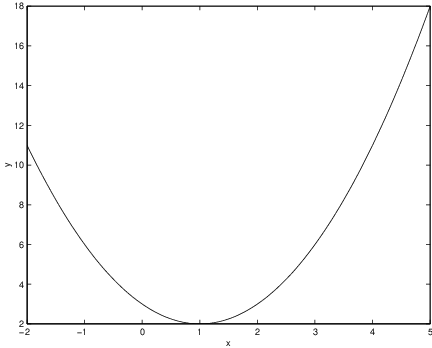
x = linspace(-2,5);
 
y = x.*x - 2*x + 3;
 
plot(x,y)

produces the graph of (??) in Figure ??.

Figure 6: Graph of $y = x^2 - 2x + 3$ .

In a similar fashion, MATLAB has the ‘dot’ operations of ./, . $\backslash$ , and .ˆ, as well as .*.

Exercises

Find the equation for the plane perpendicular to the vector $(2,3,1)$ and containing the point $(-1,-2,3)$ . The equation of the desired plane is $\answer {2}x + \answer {3}y + z = -5$ .

Note that a vector perpendicular to a plane is orthogonal to any vector connecting two points in the plane. So, if $X_0 = (-1,-2,3)$ is one point in the plane perpendicular to $N = (2,3,1)$ and $X = (x,y,z)$ is any other point in that plane, then $(X - X_0) \cdot N = 0$ . Substituting into this formula, we obtain $2(x + 1) + 3(y + 1) + 1(z - 3) = 0\quad \mbox {or}\quad 2x + 3y + z = -5.$

Determine three systems of two linear equations in two unknowns so that the first system has a unique solution, the second system has an infinite number of solutions, and the third system has no solutions.

For example, the system $\begin {array}{rrrrr} x & + & y & = & 2 \\ x & - & y & = & 0\end {array}$ has…

No solutions. Exactly one solution. Infinitely many solutions.

The system $\begin {array}{rrrrr} x & + & y & = & 2 \\ 2x & + & 2y & = & 4\end {array}$ has…

No solutions. Exactly one solution. Infinitely many solutions.

while the system $\begin {array}{rrrrr} x & + & y & = & 2 \\ x & + & y & = & 4\end {array}$ has…

No solutions. Exactly one solution. Infinitely many solutions.

Write the equation of the plane through the origin containing the vectors $(1,0,1)$ and $(2,-1,2)$ . The equation for the plane is $z = \answer {x}$ .

Note that the plane goes through the origin and contains the vectors $(1,0,1)$ and $(2,-1,2)$ , and therefore contains the points $(0,0,0)$ , $(1,0,1)$ , and $(2,-1,2)$ . The general equation for a plane is $ax + by + cz = d$ . We can substitute the coordinates of the three points into this equation to get the linear system $\begin {array}{rrrrrrr} & & & & 0 & = & d \\ a & & & + & c & = & d \\ 2a & - & b & + & 2c & = & d\end {array}$ We can solve the system by substitution to get $b = d = 0$ and $a = -c$ , which yields the equation of the plane.

Find a system of two linear equations in three unknowns whose solution set is the line consisting of scalar multiples of the vector $(1,2,1)$ .

For example, one such system is: $\begin {array}{rrrrrrr} x & - & y & + & z & = & 0 \\ \answer {2}x & + & y & - & \answer {4}z & = & 0\end {array}$

The solution set contains all multiples of the vector $(1,2,1)$ , so it contains the origin, since $0(1,2,1) = (0,0,0)$ . The equation of any plane containing the origin is $ax + by + cz = 0$ . Substituting the point $(1,2,1)$ implies that $a + 2b + c = 0$ . Any two equations which satisfy that condition and are not multiples of one another will have the appropriate line as a solution set. For example, let $(a,b,c) = (1,-1,1)$ in the first equation, and $(a,b,c) = (2,1,-4)$ in the second equation to obtain the system given here.

Find a vector $u$ normal to the plane $2x+2y+z=3$ .
$u = \left ( \answer [format=integer,id=ux]{2}, \answer [format=integer,id=uy]{2}, \answer [format=integer,id=uz]{1} \right )$
Find a vector $v$ normal to the plane $x+y+2z=4$ .
$v = \left ( \answer [format=integer,id=vx]{1}, \answer [format=integer,id=vy]{1}, \answer [format=integer,id=vz]{2} \right )$
Find the cosine of the angle $\theta$ between the vectors $u$ and $v$ . $\cos \theta = \answer {\frac {2}{\sqrt {6}}}$

Determine graphically the geometry of the set of solutions to the system of equations in the three unknowns $x,y,z$ : $\begin {array}{rcrcr} x & + & 3z & = & 1\\ 3x & - & z & = & 1\\ & & z & = & 2 \end {array}$ by sketching the plane of solutions for each equation individually. Describe in words why there are no solutions to this system. (Use MATLAB graphics to verify your sketch. Note that you should enter the last equation as z = 2 - 0*x - 0*y and the first two equations with 0*y terms. Try different views — but include view([0 1 0]) as one view.)

Use MATLAB to solve graphically the planar system of linear equations $\arraycolsep 2pt \begin {array}{rcrcr} x & + & 4y & = & -4 \\ 4x & + & 3y & = & 4 \end {array}$ to an accuracy of two decimal points.

Hint: The MATLAB command zoom on allows us to view the plot in a window whose axes are one-half those of original. Each time you click with the mouse on a point, the axes’ limits are halved and centered at the designated point. Coupling zoom on with grid on allows you to determine approximate numerical values for the intersection point.

Use MATLAB to solve graphically the planar system of linear equations $\arraycolsep 2pt \begin {array}{rcrcr} 4.23x & + & 0.023y & = & -1.1 \\ 1.65x & - & 2.81y & = & 1.63 \end {array}$ to an accuracy of two decimal points.

Use MATLAB to find an approximate graphical solution to the three dimensional system of linear equations $\begin {array}{rcrcrcr} 3x & - & 4y & + & 2z & = & -11\\ 2x & + & 2y & + & z & = & 7\\ -x & + & y & - & 5z & = & 7. \end {array}$ Then use MATLAB to find an exact solution.

Use MATLAB to determine graphically the geometry of the set of solutions to the system of equations: $\begin {array}{rcrcrcr} x & + & 3y & + & 4z & = & 5\\ 2x & + & y & + & z & = & 1\\ -4x & + & 3y & + & 5z & = & 7. \end {array}$ Attempt to use MATLAB to find an exact solution to this system and discuss the implications of your calculations.

Hint: After setting up the graphics display in MATLAB, you can use the command view([0,1,0]) to get a better view of the solution point.

Use MATLAB to graph the function $y = 2 - x\sin (x^2-1)$ on the interval $[-2,3]$ . How many relative maxima does this function have on this interval?