Recall that a planar autonomous system of ordinary differential equations has the form
Computer experiments using pplane5 always appear to find a unique solution to initial value problems. More precisely, we are led to believe that there is just one solution to (??) satisfying the initial conditionsExistence and Uniqueness of Solutions
In fact, existence and uniqueness of solutions are not always guaranteed — though they are guaranteed for a large class of differential equations, as the following theorem shows.
For example, consider the planar system of constant coefficient linear differential equations:
In (??), and . The partial derivatives of and are easy to calculate; they are: , , , and . As constant functions, all of these partial derivatives are continuous. Hence, existence and uniqueness of solutions to the initial value problem for (??) are guaranteed by Theorem ??.Although we have stated this theorem just for planar systems, the theorem itself is valid in all dimensions. For example, in one dimension the analog of Theorem ?? states that the differential equation with initial condition has a unique solution when exists and is continuous near .
A discussion of the proof of this theorem is beyond the scope of this text; nevertheless, the theorem is valid and we will use its consequences.
An Example of Nonuniqueness of Solutions
Indeed, uniqueness of solutions is not even guaranteed for single equations. Here is an example:
with the initial condition Certainly the constant function is a solution to (??) satisfying the initial value . In addition, the function is a solution to (??). This fact is checked by direct calculation:Example (??) shows that hypotheses like those in Theorem ?? are needed. Indeed, in (??) Hence, is not differentiable at and the hypotheses of Theorem ?? fail.
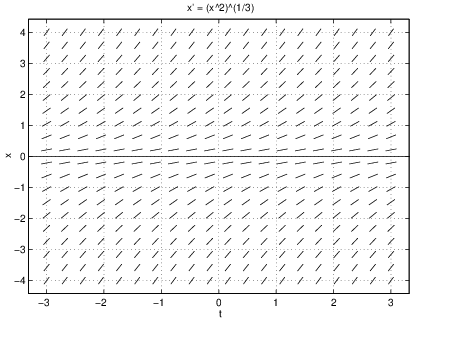
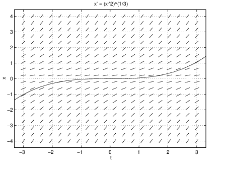
At this point it is worth looking to see what dfield5 computes numerically. Start dfield5 and change the differential equation to:
x’ = (x^2)^(1/3)Writing the differential equation in this way guarantees that the computer will not compute square roots of negative numbers. Click on the Proceed button. In the DFIELD5 Display window attempt to click on the origin — that is, attempt to enter the initial condition using the mouse. You will surely get a solution that has a similar shape to the graph of the cubic function . In the DFIELD5 Options menu click on Keyboard input, and in the DFIELD5 Keyboard input window enter the values and . After clicking on the Compute button you will see the solution . Now click on the Erase all solutions button in the DFIELD5 Options menu. Change the initial value of to in the DFIELD5 Keyboard input window and click on Compute. You will see a solution that looks like . See Figure ??.
At this stage, we do not have the background to discuss the numerical method employed by dfield5.
The Initial Value Problem for Linear Systems
In this chapter we discuss how to find solutions to (??) satisfying the initial values and . It is convenient to rewrite (??) in matrix form as:
The initial value problem is then stated as: Find a solution to (??) satisfying where . Everything that we have said here works equally well for dimensional systems of linear differential equations. Just let be an matrix and let be an vector of initial conditions.Solving the Initial Value Problem Using Superposition
In Section ?? we discussed how to solve (??) when the eigenvalues of are real and distinct. Recall that when and are distinct real eigenvalues of with associated eigenvectors and , there are two solutions to (??) given by the explicit formulas Superposition guarantees that every linear combination of these solutions is a solution to (??). In addition, we can always choose scalars to solve any given initial value problem of (??). It follows from the uniqueness of solutions to initial value problems stated in Theorem ?? that all solutions to (??) are included in this family of solutions.
We generalize this discussion so that we will be able to find closed form solutions to (??) in Section ?? when the eigenvalues of are complex or are real and equal.
Suppose that and are two solutions to (??) such that are linearly independent. The existence part of Theorem ?? guarantees that such solutions exist. Then all solutions to (??) are linear combinations of these two solutions. We verify this statement as follows. Corollary ?? of Chapter ?? states that since is a linearly independent set in , it is also a basis of . Thus for every there exist scalars such that It follows from superposition and Theorem ?? that the solution is the unique solution whose initial condition vector is .
We have proved that every solution to this linear system of differential equations is a linear combination of these two solutions — that is, we have proved that the dimension of the space of solutions to (??) is two. This proof generalizes immediately to a proof of the following theorem for systems.
We call (??) the general solution to the system of differential equations . When solving the initial value problem we find a particular solution by specifying the scalars .
Consider a special case of Theorem ??. Suppose that the matrix has linearly independent eigenvectors with real eigenvalues . Then the functions are solutions to . Corollary ?? implies that the functions form a basis for the space of solutions of this system of differential equations. Indeed, the general solution to (??) is
The particular solution that solves the initial value is found by solving (??) for the scalars .Exercises
In Exercises ?? – ??, consider the system of differential equations
In Exercises ?? – ??, consider the system of differential equations
In Exercises ?? – ??, consider the system of differential equations
In Exercises ?? – ??, consider the system of differential equations
In Exercises ?? – ??, consider the matrix
- Use pplane5 to find two independent eigendirections (and hence eigenvectors) for (??).
- Using (a), find the eigenvalues of the coefficient matrix of (??).
- Find a closed form solution to (??) satisfying the initial condition
- Study the time series of versus for the solution in (c) by comparing the graph of the closed form solution obtained in (c) with the time series graph using pplane5.