Second Order Equations

$\newenvironment {prompt}{}{} \newcommand {\Sec }[2]{\section {#1}} \newcommand {\trademark }[0]{{R\!\!\!\!\!\bigcirc }} \newcommand {\EXER }[0]{\section *{Exercises}} \newcommand {\CEXER }[0]{} \newcommand {\TEXER }[0]{} \newcommand {\R }[0]{\mbox {$\Bbb {R}$}} \newcommand {\C }[0]{\mbox {$\Bbb {C}$}} \newcommand {\Z }[0]{\mbox {$\Bbb {Z}$}} \newcommand {\N }[0]{\mbox {$\Bbb {N}$}} \newcommand {\D }[0]{\mbox {{\bf D}}} \newcommand {\setmin }[0]{\;\mbox {--}\;} \newcommand {\Matlab }[0]{{M\small {AT\-LAB}} } \newcommand {\Matlabp }[0]{{M\small {AT\-LAB}}} \newcommand {\computer }[0]{\Matlab Instructions} \newcommand {\half }[0]{\mbox {$\frac {1}{2}$}} \newcommand {\compose }[0]{\raisebox {.15ex}{\mbox {{\scriptsize $\circ $}}}} \newcommand {\AND }[0]{\quad \mbox {and}\quad } \newcommand {\vect }[2]{\left (\begin {array}{c} #1_1 \\ \vdots \\ #1_{#2}\end {array}\right )} \newcommand {\mattwo }[4]{\left (\begin {array}{rr} #1 & #2\\ #3 &#4\end {array}\right )} \newcommand {\mattwoc }[4]{\left (\begin {array}{cc} #1 & #2\\ #3 &#4\end {array}\right )} \newcommand {\vectwo }[2]{\left (\begin {array}{r} #1 \\ #2\end {array}\right )} \newcommand {\vectwoc }[2]{\left (\begin {array}{c} #1 \\ #2\end {array}\right )} \newcommand {\inv }[0]{^{-1}} \newcommand {\CC }[0]{{\cal C}} \newcommand {\CCone }[0]{\CC ^1} \newcommand {\Span }[0]{{\rm span}} \newcommand {\rank }[0]{{\rm rank}} \newcommand {\trace }[0]{{\rm tr}} \newcommand {\RE }[0]{{\rm Re}} \newcommand {\IM }[0]{{\rm Im}} \newcommand {\nulls }[0]{{\rm null\;space}} \newcommand {\dps }[0]{\displaystyle } \newcommand {\arraystart }[0]{\renewcommand {\arraystretch }{1.8}} \newcommand {\arrayfinish }[0]{\renewcommand {\arraystretch }{1.2}} \newcommand {\Start }[1]{\vspace {0.08in}\noindent {\bf Section~\ref {#1}}} \newcommand {\exer }[1]{\noindent {\bf \ref {#1}}} \newcommand {\ans }[0]{} \newcommand {\matthree }[9]{\left (\begin {array}{rrr} #1 & #2 & #3 \\ #4 & #5 & #6 \\ #7 & #8 & #9\end {array}\right )} \newcommand {\cvectwo }[2]{\left (\begin {array}{c} #1 \\ #2\end {array}\right )} \newcommand {\cmatthree }[9]{\left (\begin {array}{ccc} #1 & #2 & #3 \\ #4 & #5 & #6 \\ #7 & #8 & #9\end {array}\right )} \newcommand {\vecthree }[3]{\left (\begin {array}{r} #1 \\ #2 \\ #3\end {array}\right )} \newcommand {\cvecthree }[3]{\left (\begin {array}{c} #1 \\ #2 \\ #3\end {array}\right )} \newcommand {\cmattwo }[4]{\left (\begin {array}{cc} #1 & #2\\ #3 &#4\end {array}\right )} \newcommand {\thehelp }[0]{\thesection .\arabic {equation}} \newcommand {\matlabEquation }[0]{\let \oldtheequation \theequation \renewcommand {\theequation }{\oldtheequation *}\begin {equation}} \newcommand {\HyperFirstAtBeginDocument }[0]{\AtBeginDocument } \newcommand {\epstopdfsetup }[0]{\setkeys {ETE}} changed the theorem header of amsthm failed\MessageBreak }}} \newcommand {\GetTitleStringSetup }[0]{\setkeys {gettitlestring}} \newcommand {\Sectionformat }[2]{#1}$ $% This file was *autogenerated* from secondOrderEquations.sagetex.sage with % sagetex.py version 2015/08/26 v3.0-92d9f7a %344532e7f52e7b39b95f0768ee9abe2f% md5sum of corresponding .sage file (minus "goboom","current_tex_line",and pause/unpause lines)$

A second order constant coefficient homogeneous differential equation is a differential equation of the form:

$\begin{equation} \label{eq:soex1} \ddot{x} + b\dot{x} + ax = 0, \end{equation}$ where $a$ and $b$ are real numbers.

Newton’s Second Law

Newton’s second law of motion is a second order ordinary differential equation, and for this reason second order equations arise naturally in mechanical systems. Newton’s second law states that

$\begin{equation} \label{e:2ndlaw} F=ma \end{equation}$ where $F$ is force, $m$ is mass, and $a$ is acceleration.

Newton’s Second Law and Particle Motion on a Line

For a point mass moving along a line, (??) is

$\begin{equation} \label{E:F=ma} F=m\frac{d^2x}{dt^2}, \end{equation}$ where $x(t)$ is the position of the point mass at time $t$ . For example, suppose that a particle of mass $m$ is falling towards the earth. If we let $g$ be the gravitational constant and if we ignore all forces except gravitation, then the force acting on that particle is $F=-mg$ . In this case Newton’s second law leads to the second order ordinary differential equation $\begin{equation} \label{e:pointpart} \frac{d^2x}{dt^2}+g=0. \end{equation}$

Newton’s Second Law and the Motion of a Spring

As a second example, consider the spring model pictured in Figure ??. Assume that the spring has zero mass and that an object of mass $m$ is attached to the end of the spring. Let $L$ be the natural length of the spring, and let $x(t)$ measure the distance that the spring is extended (or compressed). It follows from Newton’s Law that (??) is satisfied. Hooke’s law states that the force $F$ acting on a spring is $F = -\kappa x,$ where $\kappa$ is a positive constant. If the spring is damped by sliding friction, then $F=-\kappa x - \mu \frac {dx}{dt},$ where $\mu$ is also a positive constant. Suppose, in addition, that an external force $F_{ext}(t)$ also acts on the mass and that that force is time-dependent. Then the entire force acting on the mass is $F=-\kappa x - \mu \frac {dx}{dt}+F_{ext}(t).$ By Newton’s second law, the motion of the mass is described by

$\begin{equation} \label{e:springeq} m\frac{d^2x}{dt^2} + \mu\frac{dx}{dt} + \kappa x = F_{ext}(t), \end{equation}$ which is again a second order ordinary differential equation.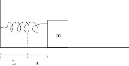

Figure 1: Hooke’s Law spring.

A Reduction to a First Order System

There is a simple trick that reduces a single linear second order differential equation to a system of two linear first order equations. For example, consider the linear homogeneous ordinary differential equation (??). To reduce this second order equation to a first order system, just set $y=\dot {x}$ . Then (??) becomes $\dot {y} + by + ax = 0.$ It follows that if $x(t)$ is a solution to (??) and $y(t)=\dot {x}(t)$ , then $(x(t),y(t))$ is a solution to

$\begin{equation} \label{e:soex1sys} \begin{array}{rcl} \dot{x} & = & y \\ \dot{y} & = & -ax - by. \end{array} \end{equation}$ We can rewrite (??) as $\dot {X} = Q X.$ where $\begin{equation} \label{e:coeffmatQ} Q = \mattwo{0}{1}{-a}{-b}. \end{equation}$ Note that if $(x(t),y(t))$ is a solution to (??), then $x(t)$ is a solution to (??). Thus solving the single second order linear equation is exactly the same as solving the corresponding first order linear system.

The Initial Value Problem

To solve the homogeneous system (??) we need to specify two initial conditions $X(0)=(x(0),y(0))^t$ . It follows that to solve the single second order equation we need to specify two initial conditions $x(0)$ and $\dot {x}(0)$ ; that is, we need to specify both initial position and initial velocity.

The General Solution

There are two ways in which we can solve the second order homogeneous equation (??). First, we know how to solve the system (??) by finding the eigenvalues and eigenvectors of the coefficient matrix $Q$ in (??). Second, we know from the general theory of planar systems that solutions will have the form $x(t)=e^{\lambda _0t}$ for some scalar $\lambda _0$ . We need only determine the values of $\lambda _0$ for which we get solutions to (??).

We now discuss the second approach. Suppose that $x(t)=e^{\lambda _0t}$ is a solution to (??). Substituting this form of $x(t)$ in (??) yields the equation $\left (\lambda _0^2 + b\lambda _0 + a\right )e^{\lambda _0t} = 0.$ So $x(t)=e^{\lambda _0t}$ is a solution to (??) precisely when $p_Q(\lambda _0)=0$ , where

$\begin{equation} \label{E:charQ} p_Q(\lambda) = \lambda^2 + b\lambda + a \end{equation}$ is the characteristic polynomial of the matrix $Q$ in (??).

Suppose that $\lambda _1$ and $\lambda _2$ are distinct real roots of $p_Q$ . Then the general solution to (??) is $x(t) = \alpha _1e^{\lambda _1t} + \alpha _2e^{\lambda _2t},$ where $\alpha _j\in \R$ .

An Example with Distinct Real Eigenvalues

For example, solve the initial value problem

$\begin{equation} \label{e:ex12} \ddot{x} + 3\dot{x} + 2x = 0 \end{equation}$ with initial conditions $x(0)=0$ and $\dot {x}(0)=-2$ . The characteristic polynomial is $p_Q(\lambda ) = \lambda ^2 + 3\lambda + 2 = (\lambda +2)(\lambda +1),$ whose roots are $\lambda _1=-1$ and $\lambda _2=-2$ . So the general solution to (??) is $x(t) = \alpha _1e^{-t} + \alpha _2e^{-2t}$ To find the precise solution we need to solve $\begin {array}{rclcl} x(0) & = & \alpha _1 + \alpha _2 & = & 0 \\ \dot {x}(0) & = & -\alpha _1 - 2\alpha _2 & = & -2 \end {array}$ So $\alpha _1 = -2$ , $\alpha _2=2$ , and the solution to the initial value problem for (??) is $x(t) = -2e^{-t} + 2e^{-2t}$

An Example with Complex Conjugate Eigenvalues

Consider the differential equation

$\begin{equation} \label{E:ex13} \ddot{x} -2\dot{x} + 5x = 0. \end{equation}$ The roots of the characteristic polynomial associated to (??) are $\lambda _1=1+2i$ and $\lambda _2=1-2i$ . It follows from the discussion in the previous section that the general solution to (??) is $x(t) = \RE \left (\alpha _1 e^{\lambda _1 t} + \alpha _2 e^{\lambda _2t}\right )$ where $\alpha _1$ and $\alpha _2$ are complex scalars. Indeed, we can rewrite this solution in real form (using Euler’s formula) as $x(t) = e^t\left (\beta _1\cos (2t) + \beta _2\sin (2t)\right ),$ for real scalars $\beta _1$ and $\beta _2$ .

In general, if the roots of the characteristic polynomial are $\sigma \pm i\tau$ , then the general solution to the differential equation is: $x(t) = e^{\sigma t}\left (\beta _1\cos (\tau t) + \beta _2\sin (\tau t)\right ).$

An Example with Multiple Eigenvalues

Note that the coefficient matrix $Q$ of the associated first order system in (??) is never a multiple of $I_2$ . It follows from the previous section that when the roots of the characteristic polynomial are real and equal, the general solution has the form $x(t) = \alpha _1 e^{\lambda _1t} + \alpha _2te^{\lambda _2t}.$

Summary

It follows from this discussion that solutions to second order homogeneous linear equations are either a linear combination of two exponentials (real unequal eigenvalues), $\alpha +\beta t$ times one exponential (real equal eigenvalues), or a time periodic function times an exponential (complex eigenvalues).

In particular, if the real part of the complex eigenvalues is zero, then the solution is time periodic. The frequency of this periodic solution is often called the internal frequency, a point that is made more clearly in the next example.

Solving the Spring Equation

Consider the equation for the frictionless spring without external forcing. From (??) we get

$\begin{equation} \label{ex:uspring} m\ddot{x} + \kappa x = 0. \end{equation}$ where $\kappa >0$ . The roots are $\lambda _1=\sqrt {\frac {\kappa }{m}}i$ and $\lambda _2=-\sqrt {\frac {\kappa }{m}}i$ . So the general solution is $x(t) = \alpha \cos (\tau t) + \beta \sin (\tau t),$ where $\tau =\sqrt {\frac {\kappa }{m}}$ . Under these assumptions the motion of the spring is time periodic with period $\frac {2\pi }{\tau }$ or internal frequency $\frac {\tau }{2\pi }$ . In particular, the solution satisfying initial conditions $x(0)=1$ and $\dot {x}(0)=0$ (the spring is extended one unit in distance and released with no initial velocity) is $x(t) = \cos (\tau t).$ The graph of this function when $\tau =1$ is given on the left in Figure ??.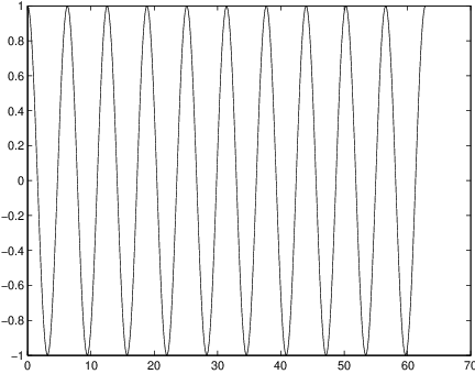

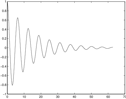
Figure 2: (Left) Graph of solution to undamped spring equation with initial conditions $x(0)=1$ and $\dot {x}(0)=0$ . (Right) Graph of solution to damped spring equation with the same initial conditions.

If a small amount of friction is added, then the spring equation is $m\ddot {x} + \mu \dot {x} +\kappa x = 0$ where $\mu >0$ is small. Since the eigenvalues of the characteristic polynomial are $\lambda =\sigma \pm i\tau$ where $\sigma = -\frac {\mu }{2m} < 0 \AND \tau =\sqrt {\frac {\kappa }{m} -\left (\frac {\mu }{2m}\right )^2},$ the general solution is $x(t) = e^{\sigma t}(\alpha \cos (\tau t) + \beta \sin (\tau t)).$ Since $\sigma <0$ , these solutions oscillate but damp down to zero. In particular, the solution satisfying initial conditions $x(0)=1$ and $\dot {x}(0)=0$ is $x(t) = e^{-\mu t/2m} \left (\cos (\tau t)-\frac {\mu }{2m\tau }\sin (\tau t)\right ).$ The graph of this solution when $\tau =1$ and $\frac {\mu }{2m}=0.07$ is given in Figure ?? (right). Compare the solutions for the undamped and damped springs.

Exercises

By direct integration solve the differential equation (??) for a point particle moving only under the influence of gravity. Find the solution for a particle starting at a height of $10$ feet above ground with an upward velocity of $20$ feet/sec. At what time will the particle hit the ground? (Recall that acceleration due to gravity is $32$ feet/sec $^2$ .)

By direct integration solve the differential equation (??) for a point particle moving only under the influence of gravity. Show that the solution is $x(t) = -\frac {1}{2}gt^2 + v_0t + x_0$ where $x_0$ is the initial position of the particle and $v_0$ is the initial velocity.

In Exercises ?? – ?? find the general solution to the given differential equation.

$\ddot {x} + 2\dot {x} - 3x = 0$ .

$\ddot {x} - 6\dot {x} + 9x = 0$ . In addition, find the solution to this equation satisfying initial values $x(1)=1$ and $\dot {x}(1)=0$ .

$\ddot {x} + 2\dot {x} + 2x = 0$ .

Prove that a nonzero solution to a second order linear differential equation with constant coefficients cannot be identically equal to zero on a nonempty interval.

Let $r>0$ and $w>0$ be constants, and let $x(t)$ be a solution to the differential equation $\ddot {x} + r\dot {x} + wx = 0.$ Show that $\dps \lim _{t\to \infty } x(t) = 0$ .

In Exercises ?? – ??, let $x(t)$ be a solution to the second order linear homogeneous differential equation (??). Determine whether the given statement is true or false.

If $x(t)$ is nonconstant and time periodic, then the roots of the characteristic polynomial are purely imaginary.

If $x(t)$ is constant in $t$ , then one of the roots of the characteristic polynomial is zero.

If $x(t)$ is not bounded, then the roots of the characteristic polynomial are equal.

Consider the second order differential equation $\begin{equation} \label{E:2ndorder} \frac{d^2x}{dt^2} + a(x)\frac{dx}{dt} + b(x) = 0. \end{equation}$ Let $y(t)=\dot {x}(t)$ and show that (??) may be rewritten as a first order coupled system in $x(t)$ and $y(t)$ as follows:

$\begin{eqnarray*} \dot{x} & = & y \\ \dot{y} & = & -b(x) - a(x) y. \end{eqnarray*}$

Use pplane5 to compute solutions to the system corresponding to the spring equations with small sliding friction. Plot the time series (in $x$ ) of the solution and observe the oscillating and damping of the solution.