Phase Portraits of Sinks

$\newenvironment {prompt}{}{} \newcommand {\Sec }[2]{\section {#1}} \newcommand {\trademark }[0]{{R\!\!\!\!\!\bigcirc }} \newcommand {\EXER }[0]{\section *{Exercises}} \newcommand {\CEXER }[0]{} \newcommand {\TEXER }[0]{} \newcommand {\R }[0]{\mbox {$\Bbb {R}$}} \newcommand {\C }[0]{\mbox {$\Bbb {C}$}} \newcommand {\Z }[0]{\mbox {$\Bbb {Z}$}} \newcommand {\N }[0]{\mbox {$\Bbb {N}$}} \newcommand {\D }[0]{\mbox {{\bf D}}} \newcommand {\setmin }[0]{\;\mbox {--}\;} \newcommand {\Matlab }[0]{{M\small {AT\-LAB}} } \newcommand {\Matlabp }[0]{{M\small {AT\-LAB}}} \newcommand {\computer }[0]{\Matlab Instructions} \newcommand {\half }[0]{\mbox {$\frac {1}{2}$}} \newcommand {\compose }[0]{\raisebox {.15ex}{\mbox {{\scriptsize $\circ $}}}} \newcommand {\AND }[0]{\quad \mbox {and}\quad } \newcommand {\vect }[2]{\left (\begin {array}{c} #1_1 \\ \vdots \\ #1_{#2}\end {array}\right )} \newcommand {\mattwo }[4]{\left (\begin {array}{rr} #1 & #2\\ #3 &#4\end {array}\right )} \newcommand {\mattwoc }[4]{\left (\begin {array}{cc} #1 & #2\\ #3 &#4\end {array}\right )} \newcommand {\vectwo }[2]{\left (\begin {array}{r} #1 \\ #2\end {array}\right )} \newcommand {\vectwoc }[2]{\left (\begin {array}{c} #1 \\ #2\end {array}\right )} \newcommand {\inv }[0]{^{-1}} \newcommand {\CC }[0]{{\cal C}} \newcommand {\CCone }[0]{\CC ^1} \newcommand {\Span }[0]{{\rm span}} \newcommand {\rank }[0]{{\rm rank}} \newcommand {\trace }[0]{{\rm tr}} \newcommand {\RE }[0]{{\rm Re}} \newcommand {\IM }[0]{{\rm Im}} \newcommand {\nulls }[0]{{\rm null\;space}} \newcommand {\dps }[0]{\displaystyle } \newcommand {\arraystart }[0]{\renewcommand {\arraystretch }{1.8}} \newcommand {\arrayfinish }[0]{\renewcommand {\arraystretch }{1.2}} \newcommand {\Start }[1]{\vspace {0.08in}\noindent {\bf Section~\ref {#1}}} \newcommand {\exer }[1]{\noindent {\bf \ref {#1}}} \newcommand {\ans }[0]{} \newcommand {\matthree }[9]{\left (\begin {array}{rrr} #1 & #2 & #3 \\ #4 & #5 & #6 \\ #7 & #8 & #9\end {array}\right )} \newcommand {\cvectwo }[2]{\left (\begin {array}{c} #1 \\ #2\end {array}\right )} \newcommand {\cmatthree }[9]{\left (\begin {array}{ccc} #1 & #2 & #3 \\ #4 & #5 & #6 \\ #7 & #8 & #9\end {array}\right )} \newcommand {\vecthree }[3]{\left (\begin {array}{r} #1 \\ #2 \\ #3\end {array}\right )} \newcommand {\cvecthree }[3]{\left (\begin {array}{c} #1 \\ #2 \\ #3\end {array}\right )} \newcommand {\cmattwo }[4]{\left (\begin {array}{cc} #1 & #2\\ #3 &#4\end {array}\right )} \newcommand {\thehelp }[0]{\thesection .\arabic {equation}} \newcommand {\matlabEquation }[0]{\let \oldtheequation \theequation \renewcommand {\theequation }{\oldtheequation *}\begin {equation}} \newcommand {\HyperFirstAtBeginDocument }[0]{\AtBeginDocument } \newcommand {\epstopdfsetup }[0]{\setkeys {ETE}} changed the theorem header of amsthm failed\MessageBreak }}} \newcommand {\GetTitleStringSetup }[0]{\setkeys {gettitlestring}} \newcommand {\Sectionformat }[2]{#1}$ $% This file was *autogenerated* from phasePortraitsOfSinks.sagetex.sage with % sagetex.py version 2015/08/26 v3.0-92d9f7a %140837c7836f1cbd79f407f54e9bf5d6% md5sum of corresponding .sage file (minus "goboom","current_tex_line",and pause/unpause lines)$

In this section we describe phase portraits and time series of solutions for different kinds of sinks. Sinks have coefficient matrices whose eigenvalues have negative real part. There are four types of sinks:

(a): spiral sink — complex eigenvalues,
(b): nodal sink — real unequal eigenvalues,
(c): focus sink — real equal eigenvalues; two independent eigenvectors, and
(d): improper nodal sink — real equal eigenvalues; one independent eigenvector.

In the previous section we showed that all solutions of sinks tend toward the origin in forward time. The way in which these solutions approach the origin distinguishes the different sink types. See Figure ??. We discuss each type of sink in turn, noting that spiral and nodal sinks are the ones that are most likely to occur.

Spiral Sinks

When the eigenvalues are complex conjugates (that is, when the coefficient matrix has no real eigenvectors), solutions spiral into the origin. This behavior can be seen from the explicit solution (??) in Chapter ??. In particular, after a similarity transformation, solutions have the form $X(t) = e^{\sigma t}\mattwo {\cos (\tau t)}{-\sin (\tau t)} {\sin (\tau t)}{\cos (\tau t)}X_0,$ where $\lambda =\sigma \pm \tau i$ are the eigenvalues of the matrix of the linear system. Since the real parts of the eigenvalues are assumed to be negative, $\sigma <0$ . Thus the initial vector $X_0$ is rotated at constant speed $\tau$ and contracted exponentially at rate $\sigma$ , and the resulting trajectory forms a spiral.

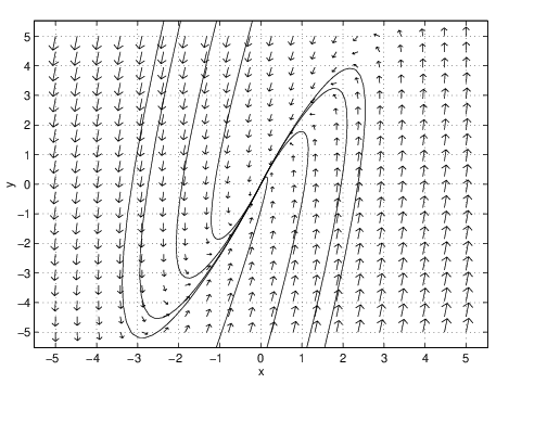
Using pplane5, we compute a typical phase portrait. Load the system

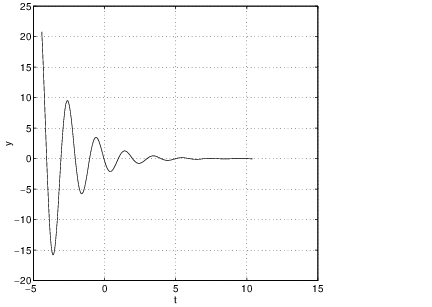
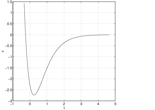
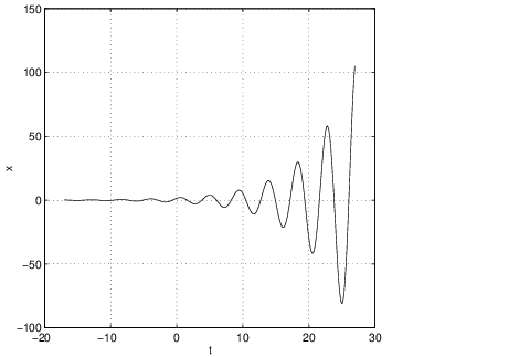
$\begin{equation} \label{e:complex2} \begin{array}{rcl} \dot{x} & = & -x + 2y \\ \dot{y} & = & -5x \end{array} \end{equation}$ into pplane5 and compute a trajectory. The result should be similar to Figure ?? (left). Note that there is no visible sign of an eigendirection in this figure. Indeed, the important feature of this phase portrait is the spiraling nature of trajectories approaching the origin. This geometric feature is typical of systems whose coefficient matrices have complex eigenvalues. In the time series, Figure ?? (right), note how the spiraling is realized as a damped oscillation.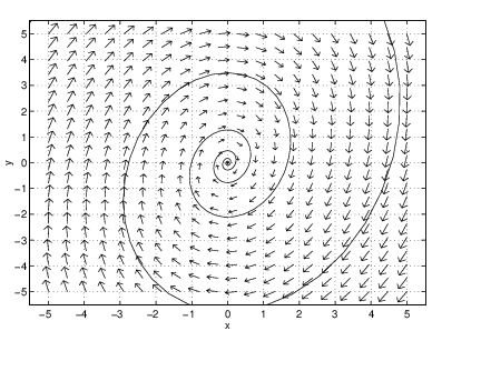

Figure 1: (Left) Phase plane for (??) for $x,y\in [-5,5]$ . (Right) Time series $y$ versus $t$ of solution

Nodal Sinks

When the eigenvalues are real and unequal, we get a nodal sink. For example, consider the differential equation

$\begin{eqnarray*} \dot{x} & = & -x+y \\ \dot{y} & = & -2y \end{eqnarray*}$

whose phase portrait is pictured in Figure ?? (left) along with the time series of one of the solution trajectories (right). Compare the time series of a solution to a nodal sink equation with the time series of the spiral sink solution given in Figure ?? (right). Note how the solution asymptotes to zero rather than oscillating about zero.

Figure 2: (Left) Phase plane of nodal sink. (Right) Time series of a typical trajectory.

Moreover, suppose that the eigenvalues are $\lambda _1 < \lambda _2 < 0$ . Then all trajectories approach the origin in forward time tangent to the eigendirection associated with the eigenvalue $\lambda _2$ . To verify this point, let $v_1$ and $v_2$ be the associated eigenvectors. Then, the general solution has the form $X(t) = \alpha _1e^{\lambda _1 t}v_1 + \alpha _2e^{\lambda _2 t}v_2 = e^{\lambda _2 t}(\alpha _1e^{(\lambda _1-\lambda _2)t}v_1 + \alpha _2v_2).$ Since $\lambda _1-\lambda _2<0$ , in forward time $X(t)$ approaches $e^{\lambda _2 t}\alpha _2v_2$ , which is tangent to the $v_2$ eigendirection. The eigenvalues in our example are $\lambda _1=-2$ and $\lambda _2=-1$ , and the eigenvector $v_2$ is just $e_1$ . Indeed, note how trajectories in the phase plane Figure ?? (left) approach the origin tangent to the $x$ -axis.

Improper Nodes

There are two types of sinks that correspond to coefficient matrices with real equal eigenvalues: those with one independent eigenvector — an improper node — and those with two independent eigenvectors — a focus.

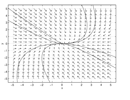
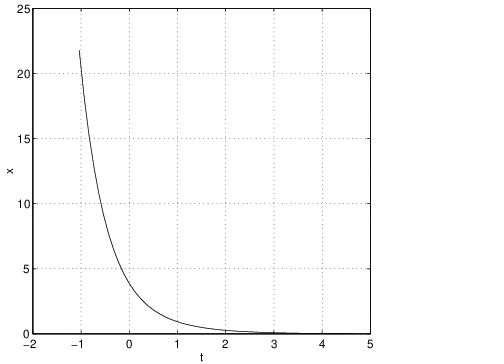
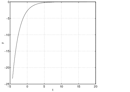
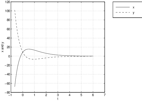
The phase plane of an improper node looks like the one pictured in Figure ?? (left) along with the time series of one of the solution trajectories (right). The equation that we use in this figure is (??). Note that trajectories approach the origin tangent to a single line — the line generated by the eigenvector. In this example, the eigenvector is approximately $(0.32,0.95)$ which generates a line through the origin of slope approximately equal to $3$ .

Figure 3: (Left) Phase plane of improper nodal sink (??). (Right) Time series of a trajectory illustrating the transient excursion away from zero.

Compare the time series of a solution to an improper nodal sink with either the time series of the spiral sink solution given in Figure ?? (right) or the nodal sink given in Figure ?? (right). Note how there is an initial excursion away from zero followed by a simple asymptote to zero. This excursion away from zero is typical of nodal sinks. To verify this point, let $\lambda _1<0$ be the eigenvalue of the coefficient matrix $C$ . Then the general solution to this equation is: $X(t) = e^{\lambda _1 t}(I_2 + tN)X_0,$ where $N = C-\lambda _1 I_2$ . The initial growth in the solution is forced by the $tN$ term. Eventually, however, exponential decay dominates and the solution approaches zero.

In addition, solutions approach zero in forward time tangent to the eigendirection spanned by the eigenvector $v$ . If we choose a generalized eigenvector $w$ so that $Nw=v$ , then we can write the general solution as $X(t) = e^{\lambda _1 t}(I_2 + tN)(\alpha v+\beta w) = e^{\lambda _1 t}\left (\alpha v + \beta w + t\beta v \right ).$ For large $t>0$ , the solution direction $\alpha v + \beta w + t\beta v$ is dominated by $t\beta v$ , and the trajectory is tangent to the $v$ eigendirection, as claimed.

Focuses

When the real equal eigenvalues correspond to a coefficient matrix $C$ having two independent eigenvectors, we have a focus. Lemma ?? of Chapter ?? states that for a focus, the matrix $C$ must be a multiple of $I_2$ ; an example of a focus is the system of differential equations

$\begin{equation} \label{e:focuseqn} \begin{array}{rcl} \dot{x} & = & -0.5x \\ \dot{y} & = & -0.5y. \end{array} \end{equation}$ The closed form solution to (??) is just $(x(t),y(t)) = e^{-0.5t}(x_0,y_0).$ So solutions remain on straight lines for all time. The phase plane for this equation is pictured in Figure ?? (left), confirming that solutions stay on lines through the origin. Algebraically, the reason for this behavior is that every line through the origin is an eigendirection. There are an infinite number of eigendirections even though there are only two independent eigenvectors.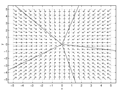

Figure 4: (Left) Phase plane of a focus. (Right) Time series of a focus.

Hyperbolic Systems

The simplest linear systems are the sinks, sources, and saddles. These linear systems all have eigenvalues that are neither zero nor purely imaginary. We call the linear system $\dot {X}=CX$ hyperbolic when all eigenvalues of $C$ have nonzero real parts.

Our discussion of phase portraits of hyperbolic linear systems is summarized in Table ??. There we reinforce the observation that the type of phase portrait is determined completely by the eigenvalues and eigenvectors of the coefficient matrix of the linear system.


NAME	EIGENVALUES

saddle	real and of opposite sign

spiral sink	complex with negative real part
spiral source	complex with positive real part

nodal sink	real, unequal, and negative
nodal source	real, unequal, and positive

improper nodal sink	real, equal, negative, and one eigenvector
improper nodal source	real, equal, positive, and one eigenvector

focus sink	real, equal, negative, and two independent eigenvectors
focus source	real, equal, positive, and two independent eigenvectors

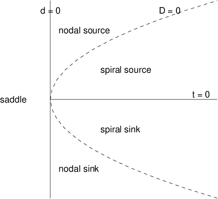
Table 1: Classification of planar hyperbolic equilibria.

Another way to determine the type of phase portrait for the hyperbolic linear system $\dot {X}=CX$ is through the determinant, trace and discriminant of $C$ . This determination can be made by answering the following four questions in order.

What is the determinant of $C$ ? $\det (C) \quad \left \{\begin {array}{ccl} < 0 & \Rightarrow & \mbox {The origin is a {\em saddle\/}. Stop.} \\ = 0 & \Rightarrow & \mbox {The system is not hyperbolic. Stop.} \\ > 0 & \Rightarrow & \mbox {Continue.} \end {array}\right .$
What is the trace of $C$ ? $\trace (C) \quad \left \{\begin {array}{ccl} < 0 & \Rightarrow & \mbox {The origin is a {\em source\/}. Continue.} \\ = 0 & \Rightarrow & \mbox {The system is not hyperbolic. Stop.} \\ > 0 & \Rightarrow & \mbox {The origin is a {\em sink\/}. Continue.} \end {array}\right .$
What is the discriminant $D$ of $C$ ? $\begin{align*} D &\equiv \trace(C)^2-4\det(C) \\ D &\quad \left\{\begin{array}{ccl} < 0 & \Rightarrow & \mbox{The origin is a {\em spiral\/}. Stop.} \\ = 0 & \Rightarrow & \mbox{The origin is a {\em node\/}. Stop.} \\ > 0 & \Rightarrow & \mbox{Continue.} \end{array}\right. \end{align*}$
Is $C$ a multiple of $I_2$ ? $\left \{\begin {array}{ccl} \text {no} & \Rightarrow & \mbox {The origin is an {\em improper node\/}. Stop.} \\ \text {yes} & \Rightarrow & \mbox {The origin is a {\em focus\/}. Stop.} \end {array}\right .$

We now verify that the answers to these four questions do indeed determine the phase portraits of hyperbolic linear systems. Recall from (??) that the determinant is the product of the eigenvalues. So if the determinant is negative, then $C$ must have one negative eigenvalue and one positive eigenvalue, and the origin is a saddle. It also follows that $C$ has a zero eigenvalue when $\det (C)=0$ , which contradicts hyperbolicity. When $\det (C)>0$ either $C$ has two real eigenvalues of the same sign or a complex conjugate pair of eigenvalues.

Next recall from (??) of Section ?? that the trace is the sum of the eigenvalues. Suppose the trace of $C$ is negative. If the eigenvalues of $C$ are real, then the two eigenvalues must be negative since they have the same sign, and the origin is a sink. If the eigenvalues are a complex conjugate pair, then the trace is twice the real part of the eigenvalues. So again the origin is a sink. A similar discussion verifies that the origin is a source when the trace of $C$ is positive. Note that $\det (C)>0$ and $\trace (C)= 0$ implies that $C$ has purely imaginary eigenvalues which contradicts the hyperbolicity of $C$ .

To understand the conclusions of question (Q3) recall from Theorem ?? of Chapter ?? that the eigenvalues of $C$ are complex conjugates when the discriminant $D$ is negative. Hence the origin is a spiral. Similarly, if $D>0$ , then the eigenvalues of $C$ are real, and the origin is a node. Finally, if $D=0$ , then the eigenvalues of $C$ are real and equal. The origin is an improper node when there is only one linearly independent eigenvector, and the origin is a focus when there are two linearly independent eigenvectors. Moreover, when a $2\times 2$ matrix has two equal eigenvalues and two linearly independent eigenvectors, it is a multiple of $I_2$ .

See Figure ?? for a classification of phase portrait types in the determinant-trace plane.

Figure 5: Classification of phase portraits in the $t$ - $d$ plane, where $t$ is the trace, $d$ is the determinant, and $D$ is the discriminant.

Exercises

For the matrix $C$ in Exercise ?? of Section ??, determine the type of phase portrait of $\dot {X}=CX$ .

In Exercises ?? – ??, find a $2\times 2$ matrix $C$ so that the given statement is satisfied.

The differential equation $\dot {X}=CX$ has a saddle at the origin with unstable orbit in the direction $(2,3)$ .

The differential equation $\dot {X}=CX$ has a spiral sink at the origin where solutions decay to the origin at rate $\sigma =-0.5$ .

The differential equation $\dot {X}=CX$ has an improper nodal source at the origin with trajectories approaching the origin tangent to the $y$ axis.

The differential equation $\dot {X}=CX$ has a nodal sink at the origin with trajectories approaching the origin tangent to the line $y=x$ .

Each picture in Figure ?? is the time series of a solution to a planar system of differential equations of the form $\dot {X}=CX$ . Describe the eigenvalues of $C$ and determine the type of planar phase for each of these systems.

Figure 6: Time series for planar systems.

In Exercises ?? – ??, use pplane5 to determine the type of phase portrait for the systems of differential equations $\dot {X}=CX$ where $C$ is the given matrix. Based on these computations answer the following questions:

Is the origin asymptotically stable?
How many real eigenvectors does the matrix $C$ have?

$C=\mattwo {\pi }{\sqrt {2}}{-1}{1}$ .

$C=\mattwo {4}{1}{6}{-1}$ .