Sinks, Saddles, and Sources

$\newenvironment {prompt}{}{} \newcommand {\Sec }[2]{\section {#1}} \newcommand {\trademark }[0]{{R\!\!\!\!\!\bigcirc }} \newcommand {\EXER }[0]{\section *{Exercises}} \newcommand {\CEXER }[0]{} \newcommand {\TEXER }[0]{} \newcommand {\R }[0]{\mbox {$\Bbb {R}$}} \newcommand {\C }[0]{\mbox {$\Bbb {C}$}} \newcommand {\Z }[0]{\mbox {$\Bbb {Z}$}} \newcommand {\N }[0]{\mbox {$\Bbb {N}$}} \newcommand {\D }[0]{\mbox {{\bf D}}} \newcommand {\setmin }[0]{\;\mbox {--}\;} \newcommand {\Matlab }[0]{{M\small {AT\-LAB}} } \newcommand {\Matlabp }[0]{{M\small {AT\-LAB}}} \newcommand {\computer }[0]{\Matlab Instructions} \newcommand {\half }[0]{\mbox {$\frac {1}{2}$}} \newcommand {\compose }[0]{\raisebox {.15ex}{\mbox {{\scriptsize $\circ $}}}} \newcommand {\AND }[0]{\quad \mbox {and}\quad } \newcommand {\vect }[2]{\left (\begin {array}{c} #1_1 \\ \vdots \\ #1_{#2}\end {array}\right )} \newcommand {\mattwo }[4]{\left (\begin {array}{rr} #1 & #2\\ #3 &#4\end {array}\right )} \newcommand {\mattwoc }[4]{\left (\begin {array}{cc} #1 & #2\\ #3 &#4\end {array}\right )} \newcommand {\vectwo }[2]{\left (\begin {array}{r} #1 \\ #2\end {array}\right )} \newcommand {\vectwoc }[2]{\left (\begin {array}{c} #1 \\ #2\end {array}\right )} \newcommand {\inv }[0]{^{-1}} \newcommand {\CC }[0]{{\cal C}} \newcommand {\CCone }[0]{\CC ^1} \newcommand {\Span }[0]{{\rm span}} \newcommand {\rank }[0]{{\rm rank}} \newcommand {\trace }[0]{{\rm tr}} \newcommand {\RE }[0]{{\rm Re}} \newcommand {\IM }[0]{{\rm Im}} \newcommand {\nulls }[0]{{\rm null\;space}} \newcommand {\dps }[0]{\displaystyle } \newcommand {\arraystart }[0]{\renewcommand {\arraystretch }{1.8}} \newcommand {\arrayfinish }[0]{\renewcommand {\arraystretch }{1.2}} \newcommand {\Start }[1]{\vspace {0.08in}\noindent {\bf Section~\ref {#1}}} \newcommand {\exer }[1]{\noindent {\bf \ref {#1}}} \newcommand {\ans }[0]{} \newcommand {\matthree }[9]{\left (\begin {array}{rrr} #1 & #2 & #3 \\ #4 & #5 & #6 \\ #7 & #8 & #9\end {array}\right )} \newcommand {\cvectwo }[2]{\left (\begin {array}{c} #1 \\ #2\end {array}\right )} \newcommand {\cmatthree }[9]{\left (\begin {array}{ccc} #1 & #2 & #3 \\ #4 & #5 & #6 \\ #7 & #8 & #9\end {array}\right )} \newcommand {\vecthree }[3]{\left (\begin {array}{r} #1 \\ #2 \\ #3\end {array}\right )} \newcommand {\cvecthree }[3]{\left (\begin {array}{c} #1 \\ #2 \\ #3\end {array}\right )} \newcommand {\cmattwo }[4]{\left (\begin {array}{cc} #1 & #2\\ #3 &#4\end {array}\right )} \newcommand {\thehelp }[0]{\thesection .\arabic {equation}} \newcommand {\matlabEquation }[0]{\let \oldtheequation \theequation \renewcommand {\theequation }{\oldtheequation *}\begin {equation}} \newcommand {\HyperFirstAtBeginDocument }[0]{\AtBeginDocument } \newcommand {\epstopdfsetup }[0]{\setkeys {ETE}} changed the theorem header of amsthm failed\MessageBreak }}} \newcommand {\GetTitleStringSetup }[0]{\setkeys {gettitlestring}} \newcommand {\Sectionformat }[2]{#1}$ $% This file was *autogenerated* from sinksSaddlesAndSources.sagetex.sage with % sagetex.py version 2015/08/26 v3.0-92d9f7a %5b85436d777c7d5b71b2569b5b4e024b% md5sum of corresponding .sage file (minus "goboom","current_tex_line",and pause/unpause lines)$

The qualitative theory of autonomous differential equations begins with the observation that many important properties of solutions to constant coefficient systems of differential equations

$\begin{equation} \label{e:C2} \frac{dX}{dt}=CX \end{equation}$ are unchanged by similarity.

Begin by noting that the origin is always an equilibrium for (??) and suppose that $C$ is a $2\times 2$ matrix. The origin for (??) is called a sink if the eigenvalues of $C$ both have negative real part and a source if the eigenvalues both have positive real part. When $C$ has one eigenvalue of each sign, the origin is called a saddle.

Now suppose that $B$ is a $2\times 2$ matrix that is similar to $C$ . Lemma ?? of Chapter ?? states that $B$ and $C$ have the same eigenvalues. It follows that if the origin is a saddle for (??), then it is a saddle for $\dot {X}=BX$ . Similar statements hold for sinks and sources.

Asymptotic Stability

We now discuss asymptotic stability of the origin in linear systems. Recall from our discussion in Section ?? that the origin is asymptotically stable if every trajectory $X(t)$ beginning at an initial condition near the origin stays near $0$ for all positive $t$ , and $\lim _{t\to \infty }X(t) = 0.$ Recall also from Lemma ?? of Chapter ?? that if $B=P\inv CP$ , then $P\inv X(t)$ is a solution to $\dot {X}=BX$ whenever $X(t)$ is a solution to (??). Since $P\inv$ is a matrix of constants that do not depend on $t$ , it follows that $\lim _{t\to \infty }X(t) = 0 \Longleftrightarrow \lim _{t\to \infty }P\inv X(t) = 0.$ So the origin is asymptotically stable for $\dot {X}=BX$ if and only if it is asymptotically stable for (??). With this observation in hand, we prove that sinks are stable.

If the eigenvalues of $C$ have negative real part, then the origin is an asymptotically stable equilibrium for (??). If one of the eigenvalues of $C$ has positive real part, then the origin is unstable.

Proof

This proof is based on the closed form of solutions given in Section ??. The remark preceding this theorem states that we need only prove this theorem for differential equations up to similarity.

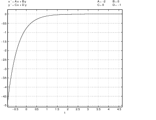
(a) If the eigenvalues $\lambda _1$ and $\lambda _2$ are real and there are two independent eigenvectors, then Chapter ??, Theorem ?? states that the matrix $C$ is similar to the diagonal matrix $B = \mattwoc {\lambda _1}{0}{0}{\lambda _2}.$ The general solution to the differential equation $\dot {X}=BX$ is $x_1(t) = \alpha _1e^{\lambda _1 t} \AND x_2(t) = \alpha _2e^{\lambda _2 t}.$ Since $\lim _{t\to \infty }e^{\lambda _1 t} = 0 = \lim _{t\to \infty }e^{\lambda _2 t},$ when $\lambda _1$ and $\lambda _2$ are negative, it follows that $\lim _{t\to \infty } X(t) = 0$ for all solutions $X(t)$ , and the origin is asymptotically stable. Note that if one of the eigenvalues, say $\lambda _1$ , is positive then $x_1(t)$ will undergo exponential growth and the origin is unstable.

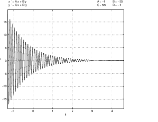
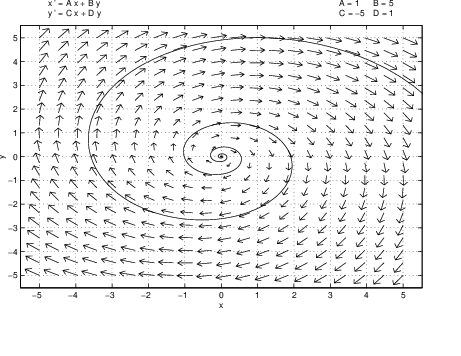
(b) If the eigenvalues of $C$ are the complex conjugates $\sigma \pm i\tau$ where $\tau \neq 0$ , then Chapter ??, Theorem ?? states that after a similarity transformation (??) has the form $\dot {X} = \mattwo {\sigma }{-\tau }{\tau }{\sigma }X,$ and solutions for this equation have the form (??) of Chapter ??, that is, $X(t) = e^{\sigma t} \mattwo {\cos (\tau t)}{-\sin (\tau t)}{\sin (\tau t)}{\cos (\tau t)}X_0 = e^{\sigma t}R_{\tau t}X_0,$ where $R_{\tau t}$ is a rotation matrix (recall (??) of Chapter ??). It follows that as time evolves the vector $X_0$ is rotated about the origin and then expanded or contracted by the factor $e^{\sigma t}$ . So when $\sigma <0$ , $\lim _{t\to \infty } X(t)=0$ for all solutions $X(t)$ . Hence the origin is asymptotically stable. Note that when $\sigma >0$ solutions spiral away from the origin.

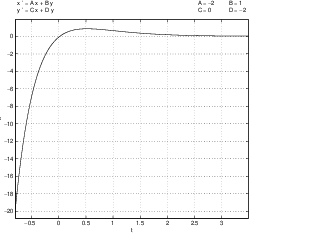
(c) If the eigenvalues are both equal to $\lambda _1$ and if there is only one independent eigenvector, then Chapter ??, Theorem ?? states that after a similarity transformation (??) has the form $\dot {X} = \mattwo {\lambda _1}{1}{0}{\lambda _1}X,$ whose solutions are $X(t) = e^{t\lambda }\mattwoc {1}{t}{0}{1} X_0$ using (??) of Chapter ??. Note that the functions $e^{\lambda _1 t} \AND te^{\lambda _1 t}$ both have limits equal to zero as $t\to \infty$ . In the second case, use l’Hôspital’s rule and the assumption that $-\lambda _1>0$ to compute $\lim _{t\to \infty } \frac {t}{e^{-\lambda _1 t}} = -\lim _{t\to \infty } \frac {1}{\lambda _1 e^{-\lambda _1 t}} = 0.$ Hence $\lim _{t\to \infty } X(t) =0$ for all solutions $X(t)$ and the origin is asymptotically stable. Note that initially $||X(t)||$ can grow since $t$ is increasing. But eventually exponential decay wins out and solutions limit on the origin. Note that solutions grow exponentially when $\lambda _1>0$ . $\blacksquare$

It is instructive to note how the time series $x_1(t)$ damps down to the origin in the three cases listed in Theorem ??. In Figure ?? we present the time series for the three coefficient matrices:

$\begin{align*} C_1 &= \mattwo{-2}{0}{0}{-1}, \\ C_2 &= \mattwo{-1}{-55}{55}{-1}, \\ C_3 &= \mattwo{-2}{1}{0}{-2}. \end{align*}$

In this figure, we can see the exponential decay to zero associated with the unequal real eigenvalues of $C_1$ ; the damped oscillation associated with the complex eigenvalues of $C_2$ ; and the initial growth of the time series due to the $te^{-2t}$ term followed by exponential decay to zero in the equal eigenvalue $C_3$ example.

Figure 1: Time series for different sinks.

Linear Stability

Saddles, sinks, and sources are distinguished by the stability of the origin. In Theorem ?? we showed that the origin is asymptotically stable if the eigenvalues have negative real part, that is, if the origin is a sink. There is another term that is commonly used and is synonymous with sink.

The origin is a linearly stable equilibrium of (??) if the eigenvalues of $C$ have negative real part.

So Theorem ?? may be restated as: linear stability implies asymptotic stability of the origin.

Sources Versus Sinks

The explicit form of solutions to planar linear systems shows that solutions with initial conditions near the origin grow exponentially in forward time when the origin of (??) is a source. We can prove this point geometrically, as follows.

The phase planes of sources and sinks are almost the same; they have the same trajectories but the arrows are reversed. To verify this point, note that

$\begin{equation} \label{e:C3} \dot{X}=-CX \end{equation}$ is a sink when (??) is a source; observe that the trajectories of solutions of (??) are the same as those of (??) — just with time running backwards. For let $X(t)$ be a solution to (??); then $X(-t)$ is a solution to (??). See Figure ?? for plots of $\dot {X}=BX$ and $\dot {X}=-BX$ where $\begin{equation} \label{E:SS} B = \mattwo{-1}{-5}{5}{-1}. \end{equation}$

So when we draw schematic phase portraits for sinks, we automatically know how to draw schematic phase portraits for sources. The trajectories are the same — but the arrows point in the opposite direction.

Figure 2: (Left) Sink $\dot {X}=BX$ where $B$ is given in (??). (Right) Source $\dot {X}=-BX$ .

Phase Portraits for Saddles

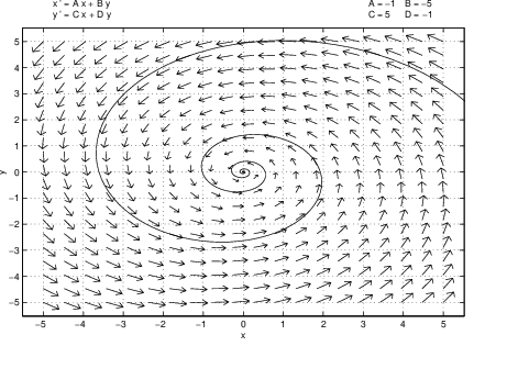
Next we discuss the phase portraits of linear saddles. Using pplane5, draw the phase portrait of the saddle

$\begin{equation} \label{e:saddlet} \begin{array}{rcl} \dot{x} & = & 2x+y\\ \dot{y} & = & -x-3y, \end{array} \end{equation}$ as in Figure ??. The important feature of saddles is that there are special trajectories (the eigendirections) that limit on the origin in either forward or backward time.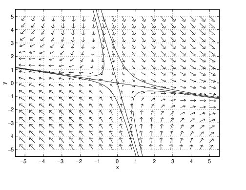

Figure 3: (Left) Saddle phase portrait. (Right) First quadrant solution time series.

The stable manifold or stable orbit of a saddle consists of those trajectories that limit on the origin in forward time; the unstable manifold or unstable orbit of a saddle consists of those trajectories that limit on the origin in backward time.

Let $\lambda _1<0$ and $\lambda _2>0$ be the eigenvalues of a saddle with associated eigenvectors $v_1$ and $v_2$ . The stable orbits are given by the solutions $X(t) = \pm e^{\lambda _1 t}v_1$ and the unstable orbits are given by the solutions $X(t) = \pm e^{\lambda _2 t}v_2$ .

Stable and Unstable Orbits using pplane5

The program pplane5 is programmed to draw the stable and unstable orbits of a saddle on command. Although the principal use of this feature is seen when analyzing nonlinear systems, it is useful to introduce this feature here. As an example, load the linear system (??) into pplane5 and click on Proceed. Now pull down the PPLANE5 Options menu and click on Find an equilibrium. Click the cross hairs in the PPLANE5 Display window on a point near the origin; pplane5 responds by opening a new window — the PPLANE5 Equilibrium point data window — and by putting a small yellow circle about the origin. The circle indicates that the numerical algorithm programmed into pplane5 has detected an equilibrium near the chosen point. A new window opens and displays the message There is a saddle point at $(0,0)$ . This window also displays the coefficient matrix (called the Jacobian for reasons that will be discussed in Section ??) at the equilibrium and its eigenvalues and eigenvectors. This process numerically verifies that the origin is a saddle (a fact that could have been verified in a more straightforward way).

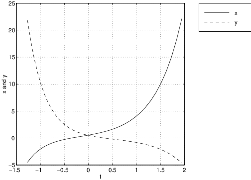
Now pull down the PPLANE5 Options menu again and click on Plot stable and unstable orbits. Next click on the mouse when the cross hairs are within the yellow circle and pplane5 responds by drawing the stable and unstable orbits. The result is shown in Figure ??(left). On this figure we have also plotted one trajectory from each quadrant; thus obtaining the phase portrait of a saddle. On the right of Figure ?? we have plotted a time series of the first quadrant solution. Note how the $x$ time series increases exponentially to $+\infty$ in forward time and the $y$ time series decreases in forward time while going exponentially towards $-\infty$ . The two time series together give the trajectory $(x(t),y(t))$ that in forward time is asymptotic to the line given by the unstable eigendirection.

Exercises

In Exercises ?? – ?? determine whether or not the equilibrium at the origin in the system of differential equations $\dot {X}=CX$ is asymptotically stable.

$C=\mattwo {1}{2}{4}{1}$ .

$C=\mattwo {-1}{2}{-4}{-1}$ .

$C=\mattwo {2}{1}{1}{-5}$ .

In Exercises ?? – ?? determine whether the equilibrium at the origin in the system of differential equations $\dot {X}=CX$ is a sink, a saddle or a source.

$C=\mattwo {-2}{2}{0}{-1}$ .

$C=\mattwo {3}{5}{0}{-2}$ .

$C=\mattwo {4}{2}{-1}{2}$ .

$C=\mattwo {8}{0}{-5}{3}$ .

$C=\mattwo {9}{-11}{-11}{9}$ .

$C=\mattwo {1}{-8}{2}{1}$ .

In Exercises ?? – ?? use pplane5 to determine whether the origin is a saddle, sink, or source in $\dot {X}=CX$ for the given matrix $C$ .

$C=\mattwoc {10}{-2.7}{4.32}{1.6}$ .

$C=\mattwoc {-10}{-2.7}{4.32}{1.6}$ .

$C=\mattwoc {-1}{2}{4.76}{1.5}$ .

$C=\mattwo {-2}{-2}{4}{1}$ .

In Exercises ?? – ?? the given matrices $B$ and $C$ are similar. Observe that the phase portraits of the systems $\dot {X}=BX$ and $\dot {X}=CX$ are qualitatively the same in two steps.

Use MATLAB to find the $2\times 2$ matrix $P$ such that $B=P\inv CP$ . Use map to understand how the matrix $P$ moves points in the plane.
Use pplane5 to observe that $P$ moves solutions of $\dot {X}=BX$ to the solution of $\dot {X}=CX$ . Write a sentence or two describing your results.

$C = \mattwo {2}{3}{-1}{-3} \AND B = \frac {1}{2}\mattwo {1}{-1}{-9}{-3}$ .

$C = \mattwo {-1}{5}{-5}{-1} \AND B = \mattwo {-1}{0.5}{-50}{-1}$ .