Wave equation on a transmission line
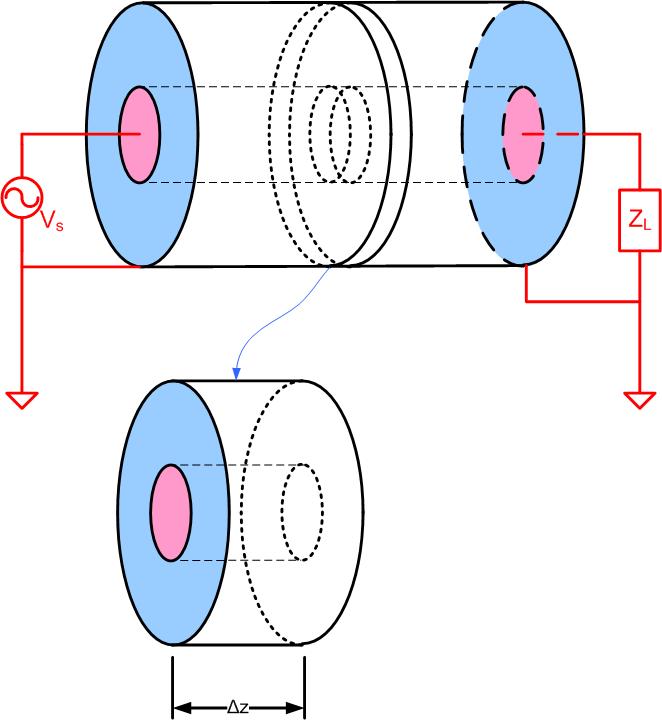
In this section, we will derive the expression for voltage and current on a transmission line. This expression will have two variables, time , and space . So far, we have only seen voltages and currents as a function of time, because all circuit elements seen so far are lumped elements. In distributed systems, we want to derive the equations for voltage and current for the case when the transmission line is longer than the fraction of a wavelength. To make sure that we do not encounter any transmission line effects to start with, we can look at the piece of a transmission line that is much smaller than the fraction of a wavelength. In other words, we cut the transmission line into small pieces to make sure there are no transmission line effects, as the pieces are shorter than the fraction of a wavelength. We then represent each piece with an equivalent circuit, as shown in Figure lineeqc (a). To derive expressions for current and voltage on the transmission line, we will use the following five-step plan
- (a)
- Look at an infinitesimal length of a transmission line .
- (b)
- Represent that piece with an equivalent circuit.
- (c)
- Write KCL, KVL for the piece in the time domain (we get differential equations)
- (d)
- Apply phasors (equations become linear)
- (e)
- Solve the linear system of equations to get the expression for the voltage and current on the transmission line as a function of .
Look at a small piece of a transmission line and represented it with an equivalent circuit. What is modeled by the circuit elements?
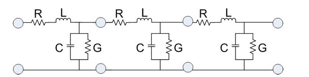
Write KVL and KCL equations for the circuit above.
KVL
KCL
Rearrange the KCL and KVL Equations te1kvl1, te1kc11 and divide them with . Equations te2kvl1, te1kc21. let and recognize the definition of the derivative Equations, te2kvl111, te1kc211.
KVL
KCL
We just derived Telegrapher’s equations in time-domain:
Telegrapher’s equations are two differential equations with two unknowns, , . It is not impossible to solve them; however, we would prefer to have linear algebraic equations. We then express time-domain variables as phasors.
are the voltage, and current anywhere on the line, and they depend on the position on the line . The Telegrapher’s equations in phasor form are
Two equations, two unknowns. To solve these equations, we first take a derivative of both equations with respect to z.
Rearange the previous equations:
Substitute Eq.te51 into Eq.te121 and Eq.te61 into Eq.te11 and we get
Or if we rearrange
The above Equations we11-we21 are called wave equations, and they represent current and voltage wave on a transmission line. is the complex propagation constant. This constant has a real and an imaginary part.
where is the attenuation constant and is the phase constant.
We can now write wave equations as:
The general solution of the second order differential equations with constant coefficients Equations eq:TLwe11 - eq:TLwe21 is:
Where represents the forward-going voltage wave, represents the reflected voltage wave, represents the forward going current wave, and represents the reflected current wave. We will see later that is the forward-going voltage wave at the load, is the reflected voltage wave at the load, is the forward going current at the load, and reflected current at the load.
In the next several sections, we will look at how to find the constants , , , , . In order to find the constants, we will introduce the concepts of transmission line impedance , reflection coefficient , input impedance .