You are about to erase your work on this activity. Are you sure you want to do this?
Updated Version Available
There is an updated version of this activity. If you update to the most recent version of this activity, then your current progress on this activity will be erased. Regardless, your record of completion will remain. How would you like to proceed?
Mathematical Expression Editor
Electric Field due to a Charge Distribution
This is an optional section.
Derive Analytical Solution for the Electric field Due to a Loop of Charge
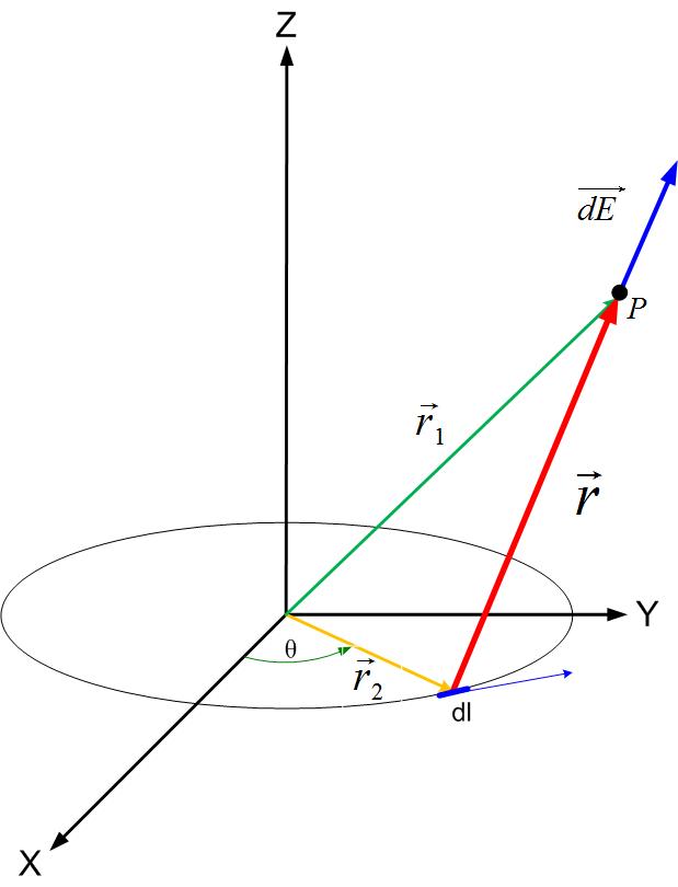
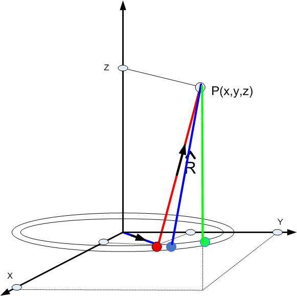
We will first find the electric field due to a loop of charge. The loop of charge is
charged with the line charge density and is in the X-Y plane, as shown in Figure fig:loopSinglePt. To
solve this problem, we first divide the loop into small pieces. The small (blue) arc
obtained in this way can be considered a point charge. The electric field
due to a point charge is shown in Figure fig:loopSinglePt(the blue arrow). The position
of the point charge is defined by a position vector . The position of point
P is defined with the position vector . The vector is defined in Equation
genfieldloop.
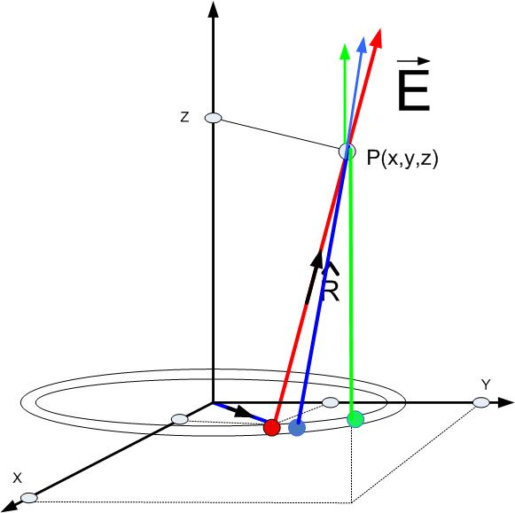
The total electric field at a point P is then equal to the sum of all the fields due to
the point charges, as shown in Figure fig:loopAllPts. The equation for the total field is given in
Equation eqtotfieldring.
Figure 1: Loop of wire uniformly charged with line charge density . Electric
field is shown due to a very small section (arc length) of the loop .
Figure 2: Loop of wire uniformly charged with line charge density . Electric
field is shown due to several very small sections (arc lengths) of the loop .
The problem now is to represent all the variables in the Equation genfieldloop ( , ,
and ) using appropriate coordinate system and given charge distribution.
The total charge on the segment is equal to . As seen in Figure fig:loopAllPts, is an arc
length in the direction of theta, , where is the radius of the loop. The vector
is the position vector of the arc length , and the vector is the position
vector of the point be of the electric field calculation. Point P is an arbitrary
point in the Cartesian coordinate system, P(x,y,z), therefore its vector is
shown in Equation eq1loop. The vector is the distance vector between the point
charge (the source) and the point at which we are calculating the electric
field.
The vector can be written in Polar Coordinates as in Equation pcvec,where is the radius
of the loop. The equation pcvec can be rewritten in Cartesian coordinate system as shown
in Equation csloopvec.
The two vectors mark the beginning and the end of the distance vector . The vector
is the sum of vectors and .
The integrals in Equations totalfieldloop4-totalfieldloop6 can be integrated analytically in some special cases only.
In general, this is in an elliptical integral and cannot be solved analytically. However,
this integral can be sold numerically.
Derive Numerical solution to the Electric Field due to a Loop of Charge
The integrals in equations totalfieldloop4-totalfieldloop6 can be represented as infinite sums using simple
numerical integration as shown in Equations totalfieldloop4n-totalfieldloop6n. Here we see that the continuous
function of was replaced with the discrete values of .
represents the length of the interval that the line is divided into, represents the
value of angle at a certain point, and designates different points on the loop. It
should be noted here that the error due to the trapezoidal rule can be improved by
using more advanced numerical integration techniques.
Matlab Code to Find the Electric Field due to a Loop of Charge
Equations totalfieldloop4n-totalfieldloop6n can be implemented in Matlab as shown below. Cut-and-paste the
program below in Matlab editor. Play with values for the size of the ring and
meshgrid values. For some values of the step, the vectors on the graph will completely
disappearcomment on why that may be.
clear all

%Specify the extents of x,y,z axes

rad=-2:1.9965:2;

%Make X,Y,Z matrices

[X Y Z]=meshgrid(rad);

%Define constants epsilon, Q. They are obviously not physical.

%They are set

%to small constants so that we get smaller numbers.

eps=1;

Q=1;

a=1;

const=Q/(2*pi*eps);

%Set the initial electric field components to zero.

Ex=0;

Ey=0;

Ez=0;

%Here we find the fieldl at all X,Y,Z points defined previously

% from each of the "unit" charges on the ring.

%th variable starts from 0.1

%to avoid the infinite value of V at the point r=1,theta=0.

for th=0.1:pi/20:2*pi


t=const./ (sqrt((X-cos(th)).^2 + (Y-sin(th)).^2 + (Z).^2)).^(3);

Ex = Ex+t.*(X-cos(th));

Ey = Ey+t.*(Y-sin(th));

Ez = Ez+t.*Z;

end

%Plot the field components Ex,Ey, Ez at points X,Y,Z.

%Scale the vectors by factor 3.

quiver3(X,Y,Z,Ex,Ey,Ez,3)

hold on;

%Plot the ring of charge where it is positioned in x-y plane.

t = linspace(0,2*pi,1000);

r=1;

x = r*cos(t);

y = r*sin(t);

plot(x,y,’b’);

hold off
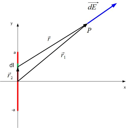
Short line of charge
Derive electric field integral, numerical solution for integral, then implement the
code in MATLAB, to find the electric field from a 1 m stick of charge, charged
with a uniform line charge density of . The stick is positioned as in Figure
stickf.
Figure 3: Stick of wire uniformly charged with line charge density . Electric
field is shown due to a very small section of the line .
In the simulation below, observe how changing the section of the selected piece of
charge (a red square) changes the field at a point P.
Then click on the play button in the lower left corner of the simulation below to
watch how each piece of charge contributes to the total electric field.
Potential
Derive Analytical Solution for the Potential Due to a Loop of Charge
Derive the potential due to a ring of charge, charged with a line charge density
.
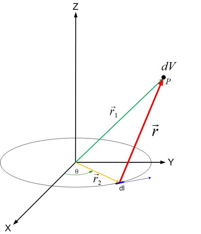
Potential due to a point charge is given in Equation genpotloop. We will first find the potential
due to a loop of charge. Assume that the loop of charge is charged with the line
charge density . The loop of charge is in the X-Y plane, as shown in Figure loopanyptf. First, we
will divide the loop into small pieces. We will assume that the small arc obtained in
this way can be considered a point charge. The potential due to a point
charge at a point P is labeled in Figure loopanyptf as . The position of the point charge
is defined by a position vector . The position of point P is defined with
the position vector . The electric scalar potential is defined in Equation
genpotloop.
Figure 4: Loop of wire uniformly charged with line charge density . Electric
field is shown due to a very small section (arc length) of the loop .
The total potential at a point P is then equal to the sum of all the potentials due to
the point charges, as shown in Figure loopanypt1. The equation for the total potential is given
in eqtotfieldringpot.
Figure 5: Loop of wire uniformly charged with line charge density . Electric
field is shown due to several very small sections (arc lengths) of the loop . Each
section is modeled by a point charge .
The problem now is to represent all the variables in the Equation genpotloop ( , , and ) using
appropriate coordinate system and given charge distribution. The total charge on the
segment is equal to . As seen in Figure loopanyptf, is an arc length in the direction of
theta (blue arrow next to ) , where is the radius of the loop. The vector
is the position vector of the arc length , and the vector is the position
vector of the point be of the electric field calculation. Point P is an arbitrary
point in the Cartesian coordinate system, P(x,y,z), therefore its vector is
shown in Equation eq1loopp. The vector is the distance vector between the point
charge (the source) and the point at which we are calculating the electric
field.
The vector can be written in Polar Coordinates as in equation pcvecp,where is the radius
of the loop. The Equation pcvecp can be rewritten in Cartesian coordinate system as in
Equation csloopvecp.
The two vectors mark the beginning and the end of the distance vector . The vector
is the sum of vectors and .
Therefore the vector’s magnitude is shown in Equations vecrloop1p.
Vector has the magnitude of:
Replacing other variables in the Equations eq1loopp-vecrloop1p to the Equation genpotloop, we get the Equation totpot
for the potential at a point P.
The integral in Equation totalfieldloopp2 can be integrated analytically in some special
cases; however, this equation can be solved numerically, as shown in the next
section.
Derive Numerical solution to the Electric Field due to a Loop of Charge
The integrals in equations totalfieldloopp2 can be represented with infinite sum using simple
numerical integration (trapezoidal rule), as shown in Equations totalfieldloop6np. Here we see
that the continuous function of was replaced with the discrete values of
.
Where represents the length of the interval that the line is divided into, represents
the value of angle at a certain point, and designates different points on the loop. It
should be noted here that the error due to the trapezoidal rule can be improved by
using more advanced numerical integration techniques.
Matlab Code to Find the Electric Potential due to a Loop of Charge
Plot the cross-section of the potential and the equipotential lines on the planes x=0,
y=0, z=0.
clear all

%Specify the extents of x,y,z axes

rad=-1.5:0.1:1.5


%Make X,Y,Z matrices

[X Y Z]=meshgrid(rad,rad,rad)

%Define constants epsilon, Q. They are obviously not physical.

%They are set

%to small constants so that we get smaller numbers.

eps=1

Q=1

const=Q/(2*pi*eps)

%Set the initial potential value to zero. Initialize V.

V=0

%Here we find the potential at all X, Y, Z points defined

% previously from

%each of the "unit" charges on the ring.

%The th variable starts from 0.1

%to avoid the infinite value of V at the point r=1,theta=0.


 for th=0.1:pi/20:2*pi

     t=const./ sqrt((X-cos(th)).^2 + (Y-sin(th)).^2 + (Z).^2)

V= V+t;

 end

%Plot the volume distribution of potential at planes

% x=0, y=0, z=0

slice(X,Y,Z,V,[0],[0],[0])

%Keep the same figure

hold on;

%Plot contours of potential at planes x=0, y=0, z=0. See

%more on contours in appendix.

h=contourslice(X,Y,Z,V,[0],[0],[0])

set(h,’EdgeColor’,’k’,’LineWidth’,1.5)
Plot several equipotential surfaces.
clear all

%Specify the extents of x,y,z axes

rad=-1.5:0.1:1.5


%Make X,Y,Z matrices

[X Y Z]=meshgrid(rad,rad,rad)


%Define constants epsilon, Q. They are obviously not physical.

%They are set

%to small constants so that we get smaller numbers.

eps=1

Q=1

const=Q/(2*pi*eps)

%Set the initial potential value to zero. Initialize V.

V=0

%Here we find the potential at all X, Y, Z points defined

%previously from

%each of the "unit" charges on the ring. The th variable

% starts from 0.1

%to avoid the infinite value of V at the point r=1,theta=0.


 for th=0.1:pi/20:2*pi

     t=const./ sqrt((X-cos(th)).^2 + (Y-sin(th)).^2 + (Z).^2)

V= V+t;

 end

%Plot the volume distribution of potential at planes

% x=0, y=0, z=0

p = patch(isosurface(X,Y,Z,V,7));

isonormals(X,Y,Z,V,p)

set(p,’FaceColor’,’red’,’EdgeColor’,’none’);

daspect([1 1 1])

view(3); axis tight

camlight

lighting gouraud
Observe the equipotential surfaces. Explain why the surfaces doughnut are shaped?
What is the electric field direction on the surface? Change the isosurface from 7 to 10
or some larger number. How does the isosurface look now? How does the potential of
a ring of charge looks at the distances far away from the ring? What about the
field?
Visualizing Scalar Fields in Matlab
To visualize scalar fields in Matlab, we can use the following functions: slice,
contourslice, patch, isonormals, camlight, and lightning. Please note that a more
detailed explanation about these functions shown here can be found in Matlab’s
help.
slice
Slice is a command that shows the magnitude of a scalar field on a plane that slices
the volume where the potential field is visualized. The format of this command is as
shown below.
slice(x,y,z,v,xslice,yslice,zslice)
Where X, Y, and Z are coordinates of points where the scaler function is
calculated, V is v the scalar function at those points, and the last three
vectors xslice, yslice, and zslice are showing where will the volume will be
sliced.
An example of slice command is given below. In the example below, there is an
additional command colormap that colors the volume with a specific palette. To see
more about different color maps, see Matlab’s help. xslice has three points at which
the x-axis will be slice. They are -1.2, .8, 2. This means that the volume will be slice
with a plane that is perpendicular to the x-axis, and it crosses the x-axis at points
-1.2, .8, and 2.
Contourslice command will display equipotential lines on a plane being the volume
where the potential field is visualized. An example of a contourslice function is shown
below.
[x,y,z] = meshgrid(-2:.2:2,-2:.25:2,-2:.16:2);

v = x.*exp(-x.^2-y.^2-z.^2); % Create volume data

[xi,yi,zi] = sphere; % Plane to contour

contourslice(x,y,z,v,xi,yi,zi)

view(3)
patch
Patch command creates a patch of color.
isonormals
Command isonormals create equipotential surfaces.
camlight
camlight(’headlight’) creates a light at the camera position.


camlight(’right’) creates a light

right and up from camera.


camlight(’left’) creates a light

left and up from camera.camlight with no arguments is the

same as camlight(’right’).


camlight(az,el) creates a light

at the specified azimuth (az) and elevation (el)

with respect to the camera position.


The camera target is the center of rotation,

and az and el are in degrees.