Brief review of impedance and admittance
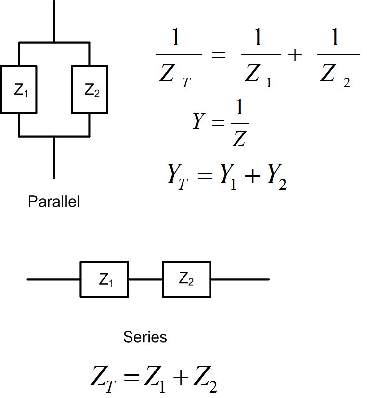
Impedance’s real part is called resistance , and the imaginary part is called reactance . It is easier to add impedances when elements are in series; see Figure fig:SCDerimpadmtrans. To find the total impedance, we add resistances and reactances separately.
The real part of an admittance is called conductance G, and the imaginary part is called susceptance B. It is easier to add admittances when elements are in parallel; see Figure fig:SCDerimpadmtrans. When adding two admittances, we add conductances and susceptances separately.
Smith Chart in Figure fig:SCDerscadmimp has impedance circles, and impedance coordinates on it. We can use this Smith Chart to read off the values for the impedance, and reflection coefficient. In the next section, we will learn to use impedance/admittance (Z/Y) Smith Chart, where both impedance and admittance circles are shown. We will use the Z/Y Smith Chart when we add impedances or admittances in parallel or series, which is useful in impedance matching that we will talk about in the next chapter.
Impedance on the Smith Chart
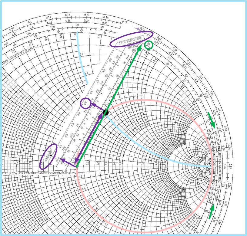
Figure fig:SCDerscimpedance, shows how to find the location of normalized impedance on the Smith Chart. is at a point where the circle of constant resistance crosses the circle of constant reactance . Figure fig:SCDerscgammafromZ shows how to find the reflection coefficient if normalized load impedance is given. Measure the distance between the origin and the point using the scale ”Reflection Coefficient E or I” on the Smith Chart’s bottom to find the reflection coefficient’s magnitude. To find the reflection coefficient’s angle, we read the scale ”Angle of Reflection Coefficient” on the Smith Chart’s perimeter, shown in green. The reflection coefficient is therefore , which is close to the actual value . If we use a ruler and compass, and a nicely sharpened pencil, we will get exactly the right answer. Try it out!
Admittance on the impedance Smith Chart
The reflection coefficient can be found from impedance or admittance. To find the reflection coefficient from impedance, we use the formula that we previously derived, where is the load impedance, and is the normalized load impedance.
Admittance is defined as , and the transmission-line admittance is defined as . If we now replace the impedances in the equation above with admittances, we get
Where is the load admittance and , is the normalized load admittance. Note that the Smith Chart shown in Figure fig:SCDerscimpedance shows circles for the impedance of the load. Therefore, the true reflection coefficient of the load is at the position of the load. We have defined above to see the position of admittance on the impedance Smith Chart.
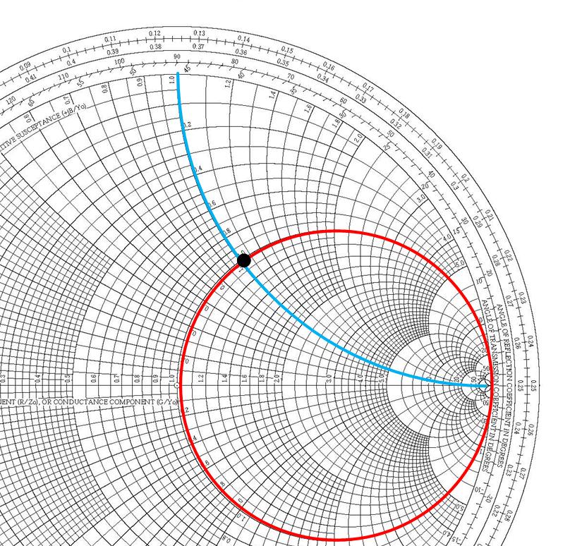
From the above Equation eq:GammaAdm, we can see that the reflection coefficient for the admittance (and the admittance) on the impedance Smith chart has the same magnitude as the load reflection coefficient. The is on the same SWR circle as the , but it is shifted with respect to the load reflection coefficient. phase shift in reflection coefficient with the same magnitude can be found in two ways:
- (a)
- by rotating the reflection coefficient for on the SWR circle to read the admittance of the load. Effectively, this means that you can draw a line through the load impedance and the center of the Smith Chart, and find the position of this line that crosses the SWR circle, away. This method’s disadvantage is that the point representing admittance changes place on the Smith Chart, depending on whether we are reading admittance or impedance. This method is used in some books, see, for example, Ulaby, Applied Electromagnetics.
- (b)
- Another way to read the admittances on the Smith chart is to use
combination of impedance/admittance (Z/I) chart, Figure fig:SCDerscadmimp1. To make the
Z/Y chart, we rotate the impedance Smith Chart for to get the admittance
point at the same position as the impedance point. Then, the impedance,
admittance, and reflection coefficient are all at the same point, but we
have to read the two scales, the impedance and admittance scale. The
disadvantage of this method is that the Z/Y Smith Chart has more circles
to read. However, this method is conceptually more straightforward, as
the point on the Smith Chart does not change position, depending on
whether we are reading admittance or impedance. The point is fixed, and
we just read the different circles. We will use this method in our class. The
example below discusses this method further.
- Solution:
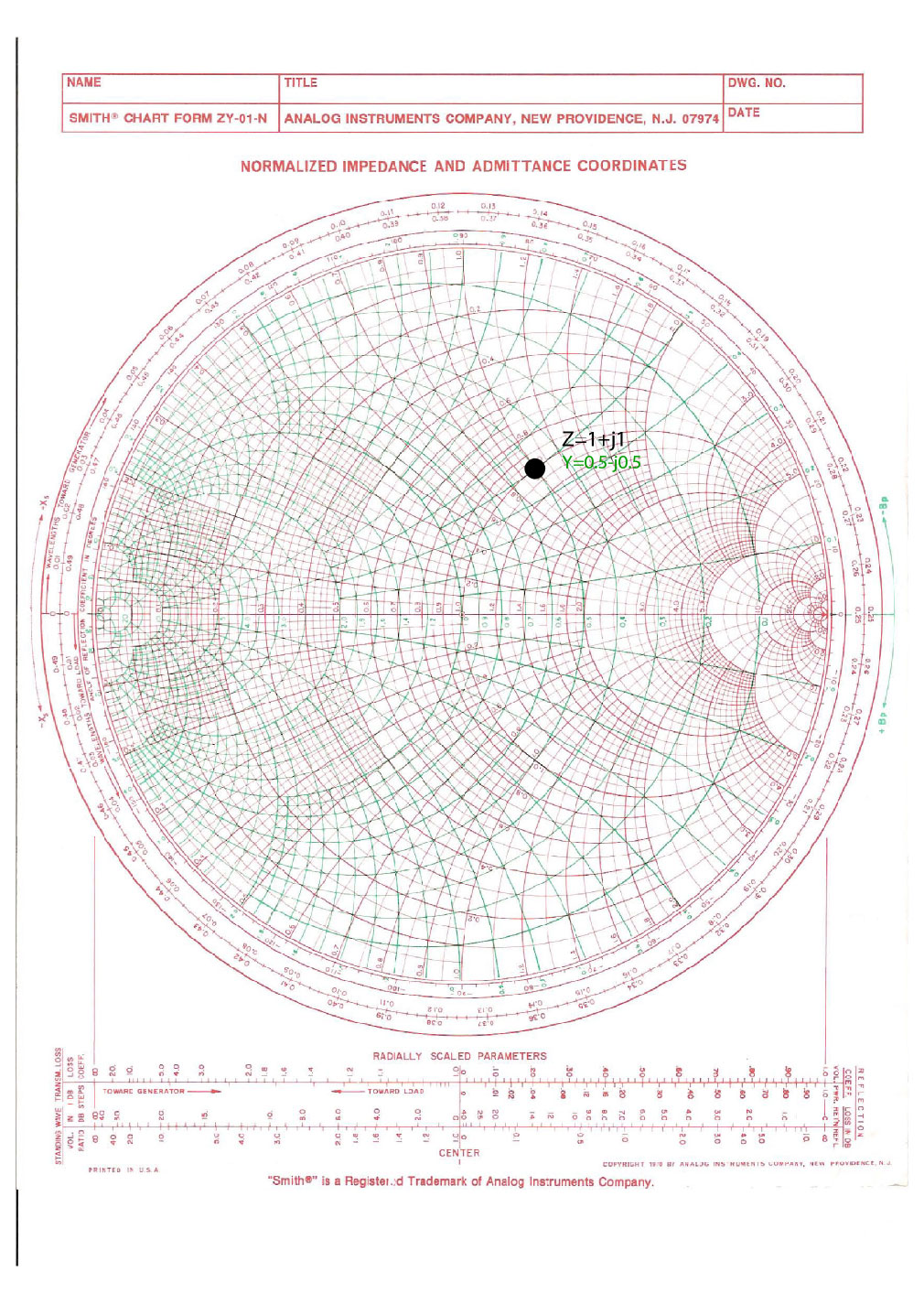
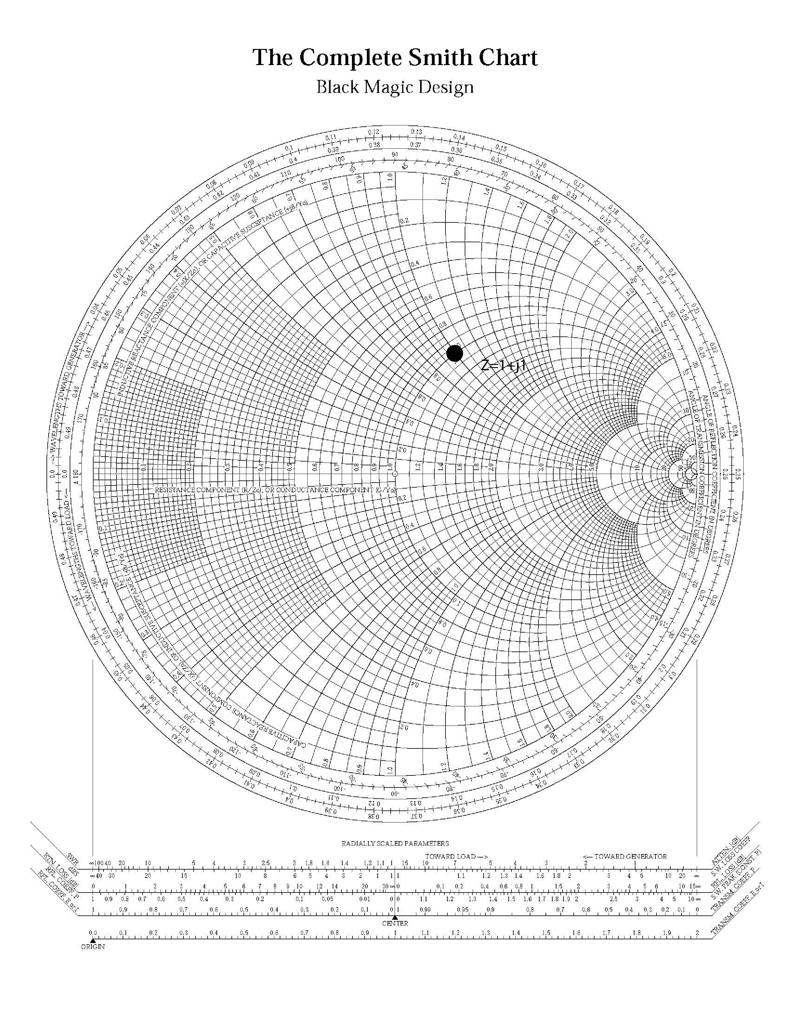
- The normalized admittance to impedance is .

The impedance is shown on the Smith Chart in Figure fig:SC1-imp.
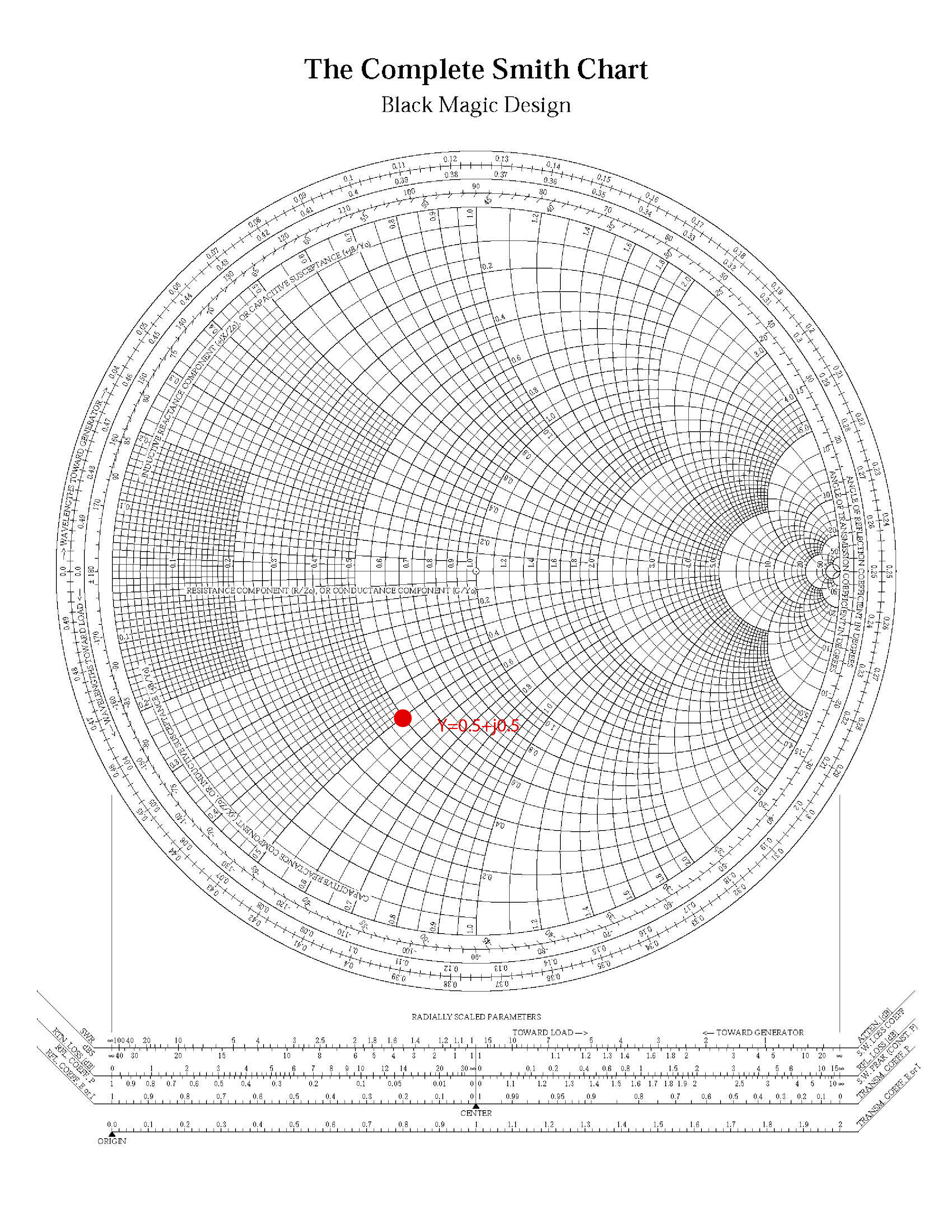
The admittance is shown on Smith Chart in Figure fig:SC1-adm. If we now use this Smith Chart and rotate it for (upside down), and place it over the chart above, we will see that the impedance and admittance point are in the same position on the Smith Chart. We call this Smith Chart a z/y Smith Chart.
Both impedance and admittance are at the same position on the z/y Smith Chart in Figure fig:SC1-both. We see two sets of circles on this chart, the red ones represent impedance circles, and the green ones represent admittance circles. To read the impedance of the point shown on the Smith Chart, we read the impedance circle scale, and to read the admittance, we read the admittance circle scales.