- a.
- By experimenting with the value of , find a value of so that the graph of appears to align with the graph of . What is the value of ?
- b.
- Similarly, experiment to find a value of so that the graph of appears to align with the graph of . What is the value of ?
- c.
- For the value of you determined in (a), compute . What do you observe?
- d.
- For the value of you determined in (b), compute . What do you observe?
- e.
- Given any exponential function of the form , do you think it’s possible to find a value of to that is the same function as ? Why or why not?
Motivating Questions
- Why can every exponential function of form (where and ) be thought of as a horizontal scaling of a single special exponential function?
- What is the natural base and what makes this number special?
Introduction
We have observed that the behavior of functions of the form is very consistent, where the only major differences depend on whether or . Indeed, if we stipulate that , the graphs of functions with different bases look nearly identical, as seen in the plots of , , , and below.

Open a new Desmos worksheet and define the following functions: , , , and .
After you define , accept the slider for , and set the range of the slider to be
.
The natural base
In the exploration above, we found that it appears possible to find a value of so that given any base , we can write the function as the horizontal scaling of given by
It’s also apparent that there’s nothing particularly special about “”: we could similarly write any function as a horizontal scaling of or , albeit with a different scaling factor for each. Thus, we might also ask: is there a best possible single base to use?Through the central topic of the rate of change of a function, calculus helps us decide which base is best to use to represent all exponential functions. While we study average rate of change extensively in this course, in calculus there is more emphasis on the instantaneous rate of change. In that context, a natural question arises: is there a nonzero function that grows in such a way that its height is exactly how fast its height is increasing?
Amazingly, it turns out that the answer to this questions is “yes,” and the function with this property is the exponential function with the natural base, denoted . The number (named in homage to the great Swiss mathematician Leonard Euler (1707-1783)) is complicated to define. Like , is an irrational number that cannot be represented exactly by a ratio of integers and whose decimal expansion never repeats. Advanced mathematics is needed in order to make the following formal definition of .
For instance, is an approximation of generated by taking the first terms in the infinite sum that defines it. Most calculators know the number and we will normally work with this number by using technology appropriately.
Initially, it’s important to note that , and thus we expect the function to lie between and . The following table gives decimal approximations to the values of , , and .
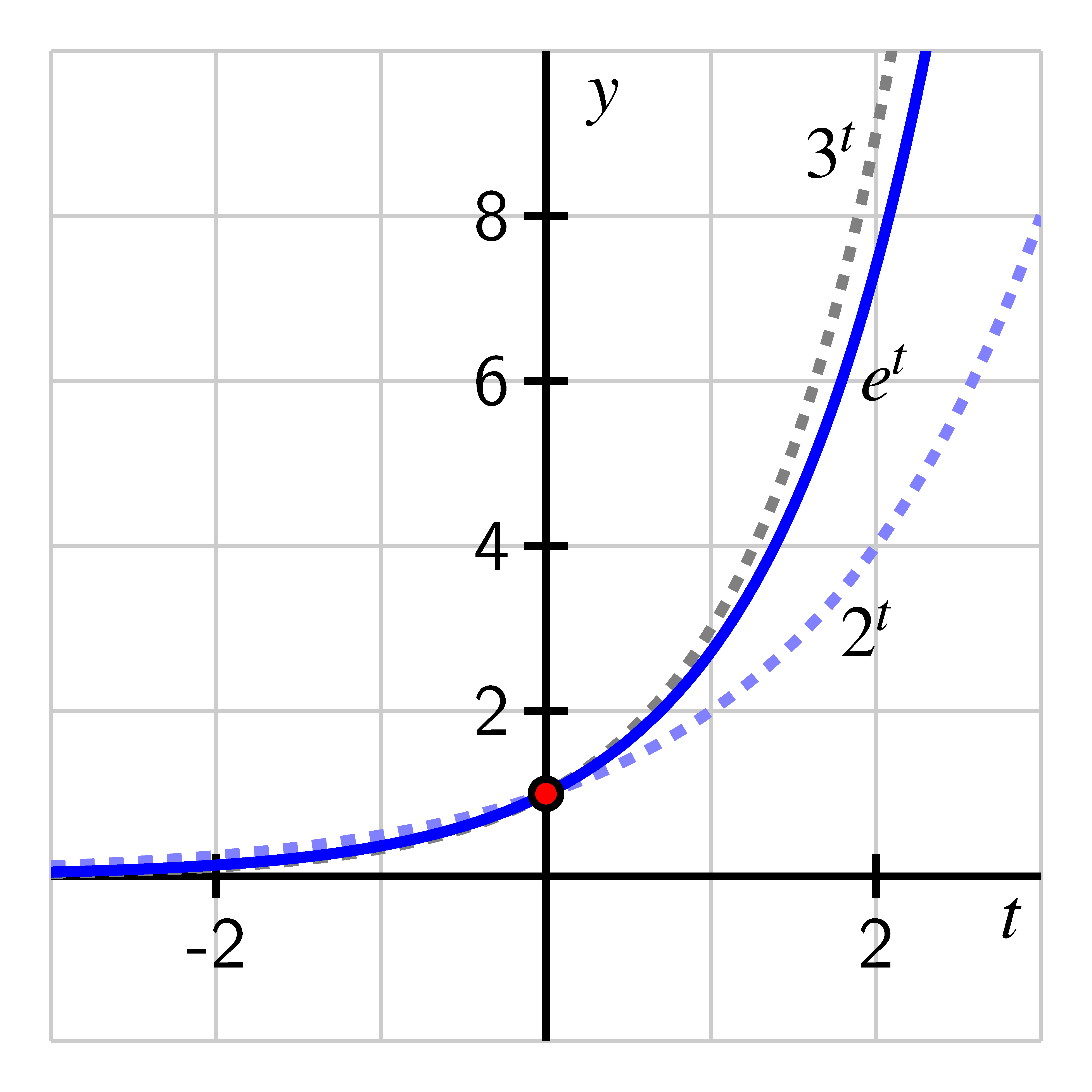
If we compare the graphs and some selected outputs of each function, as in the table and figure above, we see that the function satisfies the inequality
for all positive values of . When is negative, we can view the values of each function as being reciprocals of powers of , , and . For instance, since , it follows , or Thus, for any , Like and , the function passes through is always increasing and always concave up, and its range is the set of all positive real numbers. Recall that the average rate of change of a function on an interval
is
In this activity we explore the average rate of change of near the points where and
.
In a new Desmos worksheet, let and define the function by the rule
- a.
- What is the meaning of in terms of the function and its graph?
- b.
- Compute the value of for at least difference values of that are close to 1, both above and below 1. For instance, one value to try might be . Record a table of your results.
- c.
- What do you notice about the values you found in (b)? How do they compare to an important number?
- d.
- Explain why the following sentence makes sense: “The function is increasing at an average rate that is about the same as its value on small intervals near .”
- e.
- Adjust your definition of in Desmos by changing to so that How does the value of for values of near 2 compare to ?
Earlier, we saw graphical evidence that any exponential function can be written as a horizontal scaling of the function , plus we observed that there wasn’t anything particularly special about . Because of the importance of in calculus, we will choose instead to use the natural exponential function, as the function we scale to generate any other exponential function . We claim that for any choice of (with ), there exists a horizontal scaling factor such that .
By the rules of exponents, we can rewrite this last equation equivalently as
Since this equation has to hold for every value of , it follows that . Thus, our claim that we can scale to get requires us to show that regardless of the choice of the positive number , there exists a single corresponding value of such that .Given , we can always find a corresponding value of such that because the function passes the Horizontal Line Test, as seen in the figure below.

In this figure, we can think of as a point on the positive vertical axis. From there, we draw a horizontal line over to the graph of , and then from the (unique) point of intersection we drop a vertical line to the -axis. At that corresponding point on the -axis we have found the input value that corresponds to . We see that there is always exactly one such value that corresponds to each chosen because is always increasing, and any always increasing function passes the Horizontal Line Test.
It follows that the function has an inverse function, and hence there must be some other function such that writing is the same as writing . This important function will be be developed more later and will enable us to find the value of exactly for a given . For now, we are content to work with these observations graphically and to hence find estimates for the value of .
By graphing and appropriate horizontal lines, estimate the solution to each of the
following equations. Note that in some parts, you may need to do some algebraic
work in addition to using the graph.
- a.
- b.
- c.
- d.
- e.
- f.
- Any exponential function can be viewed as a horizontal scaling of because there exists a unique constant such that is true for every value of . This holds since the exponential function is always increasing, so given an output there exists a unique input such that , from which it follows that .
- The natural base is the special number that defines an increasing exponential function whose rate of change at any point is the same as its height at that point, a fact that is established using calculus. The number turns out to be given exactly by an infinite sum and approximately by .