You are about to erase your work on this activity. Are you sure you want to do this?
Updated Version Available
There is an updated version of this activity. If you update to the most recent version of this activity, then your current progress on this activity will be erased. Regardless, your record of completion will remain. How would you like to proceed?
Mathematical Expression Editor
Motivating Questions
What does it mean to say that a function is “exponential”?
How much data do we need to know in order to determine the formula for
an exponential function?
Are there important trends that all exponential functions exhibit?
Introduction
Linear functions have constant average rate of change and model many important
phenomena. In other settings, it is natural for a quantity to change at a rate that is
proportional to the amount of the quantity present. For instance, whether you put $
or $ or any other amount in a mutual fund, the investment’s value changes at a rate
proportional the amount present. We often measure that rate in terms of the annual
percentage rate of return.
Suppose that a certain mutual fund has a % annual return. If we
invest $, after year we still have the original $, plus we gain % of $,
so
If we instead invested $, after year we again have the original $, but now we gain % of $, and
thus
We therefore see that regardless of the amount of money originally invested, say , the
amount of money we have after year is .
If we repeat our computations for the second year, we observe
that
The ideas are identical with the larger dollar value,
so
and we see that if we invest dollars, in years our investment will grow to
.
Of course, in years at %, the original investment will have grown to . Here we see a
new kind of pattern developing: annual growth of % is leading to powers of the base ,
where the power to which we raise corresponds to the number of years the
investment has grown. We often call this phenomenon exponential growth.
Suppose that at age you have $ and you can choose between one of two
ways to use the money: you can invest it in a mutual fund that will, on
average, earn % interest annually, or you can purchase a new automobile that
will, on average, depreciate % annually. Let’s explore how the changes over
time.
Let denote the value of the $ after years if it is invested in the mutual fund, and let
denote the value of the automobile years after it is purchased.
a.
Determine , , , and .
b.
Note that if a quantity depreciates % annually, after a given year, % of
the quantity remains. Compute , , , and .
c.
Based on the patterns in your computations in (a) and (b), determine
formulas for and .
d.
Use Desmos to define and . Plot each function on the interval and record your
results on the axes below, being sure to label the scale on the axes. What
trends do you observe in the graphs? How do and compare?
Exponential functions of form
In the exploration above, we encountered the functions and that had the same basic
structure. Each can be written in the form where and are positive constants and .
Based on our earlier work with transformations, we know that the constant is a
vertical scaling factor, and thus the main behavior of the function comes from , which
we call an “exponential function”.
Let be a real number such that and . We call the
function defined by
an exponential function with base .
For an exponential function , we note that , so an exponential function of this form
always passes through . In addition, because a positive number raised to any power is
always positive (for instance, and ), the output of an exponential function is also
always positive.
In particular, is never zero and thus has no -intercepts.
Because we will be frequently interested in functions such as and with the form , we
will also refer to functions of this form as “exponential”, understanding that
technically these are vertical stretches of exponential functions according to our
definition of exponential function. In the exploration above, we found that and . It is
natural to call the “growth factor” of and similarly the growth factor of . In
addition, we note that these values stem from the actual growth rates: for and for ,
the latter being negative because value is depreciating.
In general, for a function of form , we call the growth factor. Moreover, if , we call
the growth rate. Whenever , we often say that the function is exhibiting
exponential growth, whereas if , we say exhibits exponential decay.
Suppose that at age you have $ and you can choose between one of two
ways to use the money: you can invest it in a mutual fund that will, on
average, earn % interest annually, or you can purchase a new automobile that
will, on average, depreciate % annually. Let’s explore how the changes over
time.
Let denote the value of the $ after years if it is invested in the mutual fund, and let
denote the value of the automobile years after it is purchased.
a.
What is the domain of ?
b.
What is the range of ?
c.
What is the -intercept of ?
d.
How does changing the value of affect the shape and behavior of the graph
of ? Write several sentences to explain.
e.
For what values of the growth factor is the corresponding growth rate
positive? For which -values is the growth rate negative?
f.
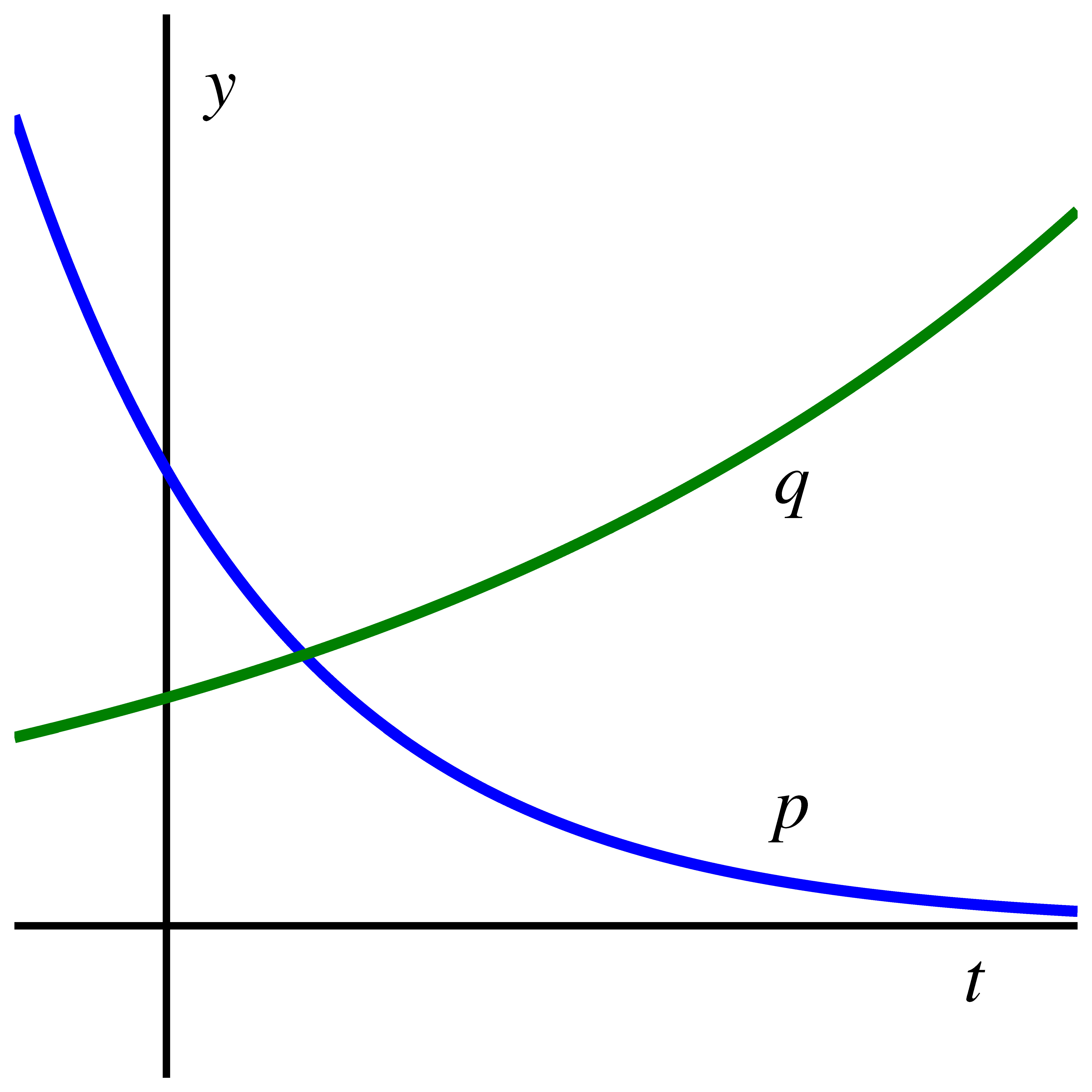
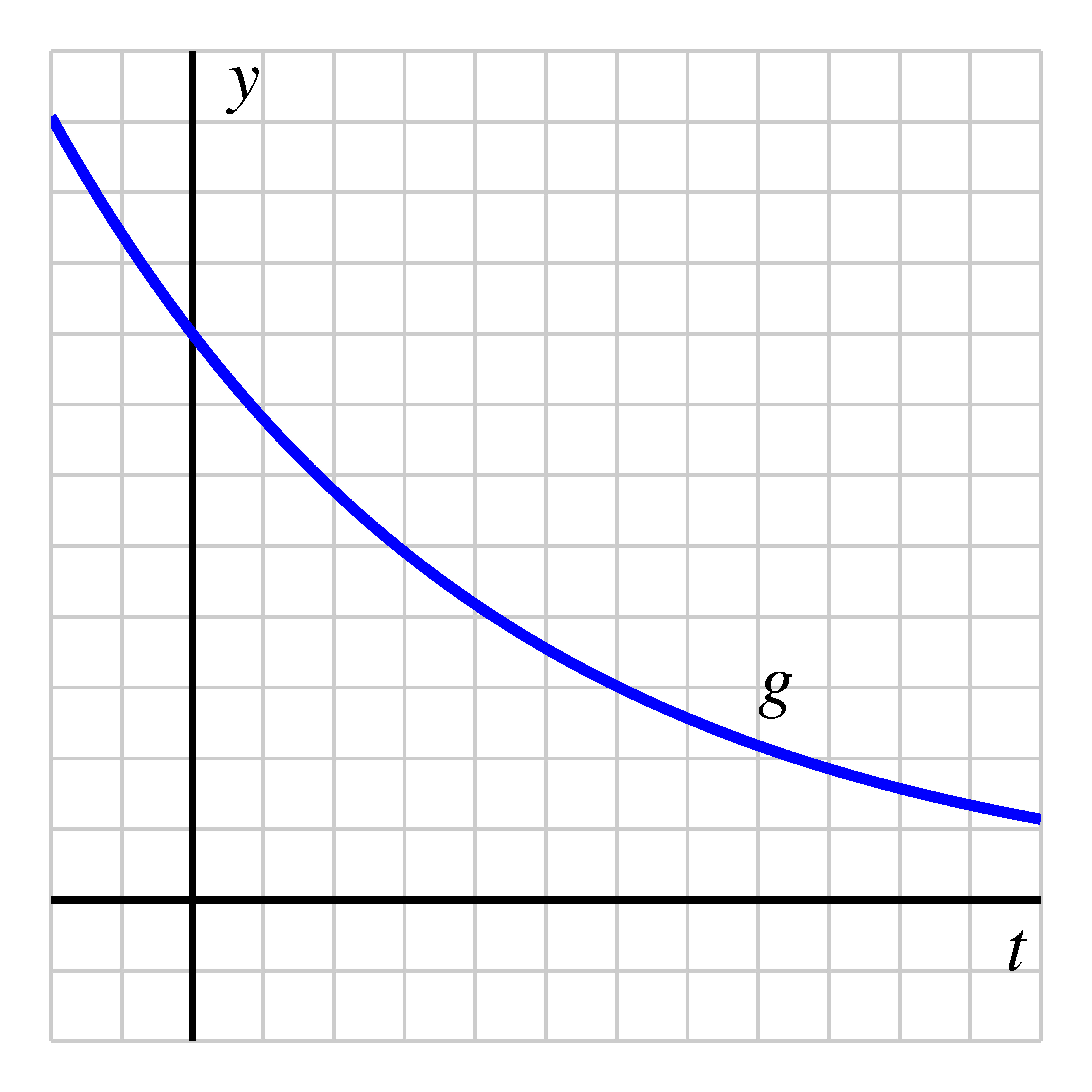
Consider the graphs of the exponential functions and provided in the figure
below. If and , what can you say about the values , , , and (beyond the fact
that all are positive and and )? For instance, can you say a certain value
is larger than another? Or that one of the values is less than ?
Determining formulas for exponential functions
To better understand the roles that and play in an exponential function,
let’s compare exponential and linear functions. In the tables below, we see
output for two different functions and that correspond to equally spaced
input.
In the leftside table for , we see a function that exhibits constant average rate of
change since the change in output is always for any change in input of . Said
differently, is a linear function with slope . Since its -intercept is , the function’s
formula is .
In contrast, the function given by rightside table for does not exhibit
constant average rate of change. Instead, another pattern is present. Observe
that if we consider the ratios of consecutive outputs in the table, we see
that
So, where the differences in the outputs in the table for are constant, the ratios in
the outputs in the table for are constant. The latter is a hallmark of exponential
functions and may be used to help us determine the formula of a function for which
we have certain information.
A function growing exponentially doesn’t just mean that it grows faster and faster,
but that the ratio between outputs corresponding to equally-spaced inputs is
constant.
If we know that a certain function is linear, it suffices to know two points that lie on
the line to determine the function’s formula. It turns out that exponential functions
are similar: knowing two points on the graph of a function known to be exponential is
enough information to determine the function’s formula. In the following example, we
show how knowing two values of an exponential function enables us to find both and
exactly.
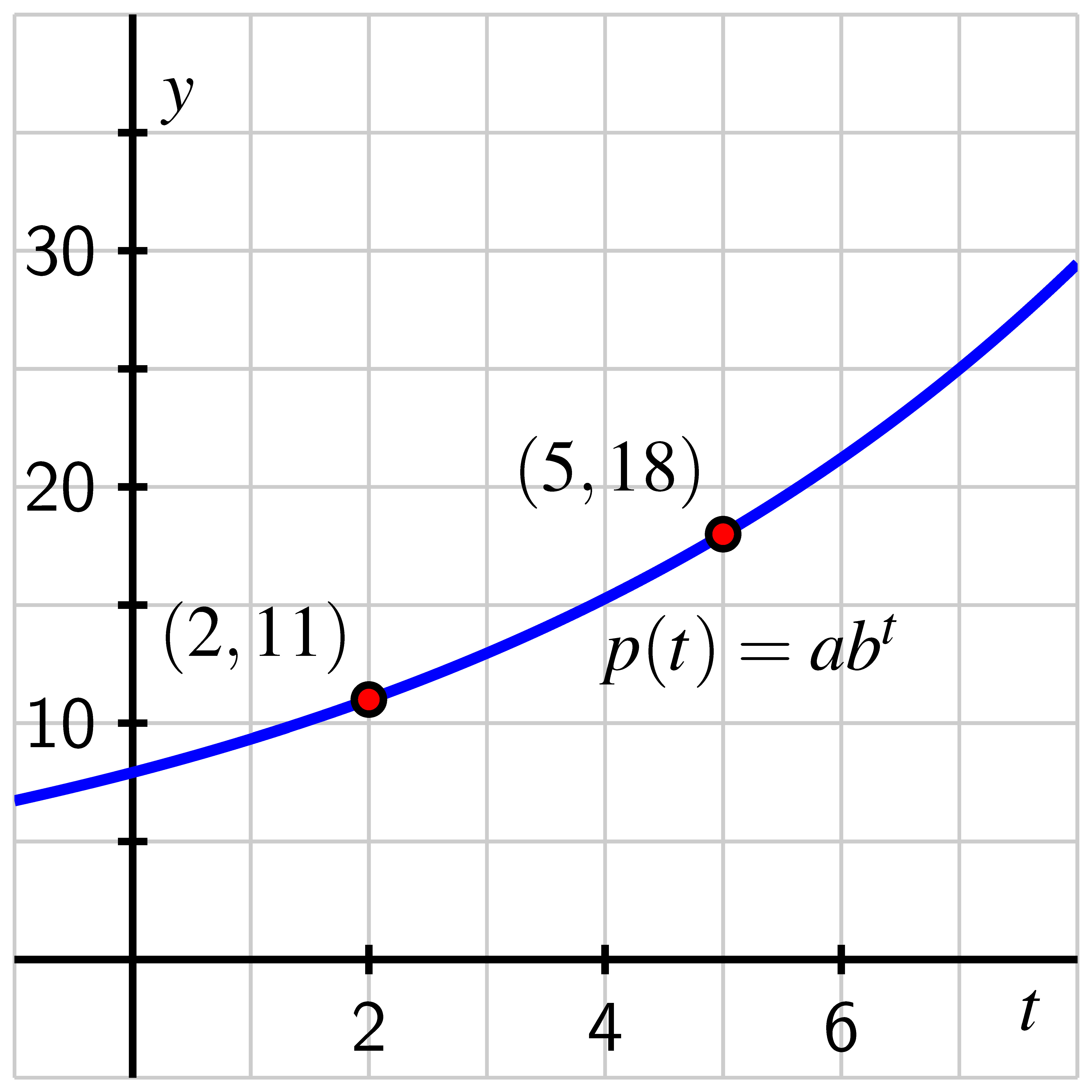
Suppose that is an exponential function and we know that and . Determine the
exact values of and for which .
Since we know that , the two data points give us two equations in the unknowns and
. First, using ,
and using we also have
Because we know that the quotient of outputs of an exponential function corresponding
to equally-spaced inputs must be constant, we thus naturally consider the quotient .
Using and , it follows that
Simplifying the fraction on the right, we see that . Solving for , we find that is the
exact value of . Substituting this value for in , it then follows that , so .
Therefore,
and a plot of confirms that the function indeed passes through and as shown in the
figure below.
The value of an automobile is depreciating. When the car is years old, its value is $;
when the car is years old, its value is $.
a.
Suppose the car’s value years after its purchase is given by the function
and that is exponential with form . What are the exact values of and ?
b.
Use the exponential model determined in (a), determine the purchase value
of the car and estimate when the car will be worth less than $1000.
c.
Suppose instead that the car’s value is modeled by a linear function and
satisfies the values stated at the outset of this activity. Find a formula for
and determine both the purchase value of the car and when the car will
be worth $.
d.
Which model do you think is more realistic? Why?
Recall that a function is increasing on an interval if its value always increasing as we
move from left to right. Similarly, a function is decreasing on an interval provided
that its value always decreases as we move from left to right.
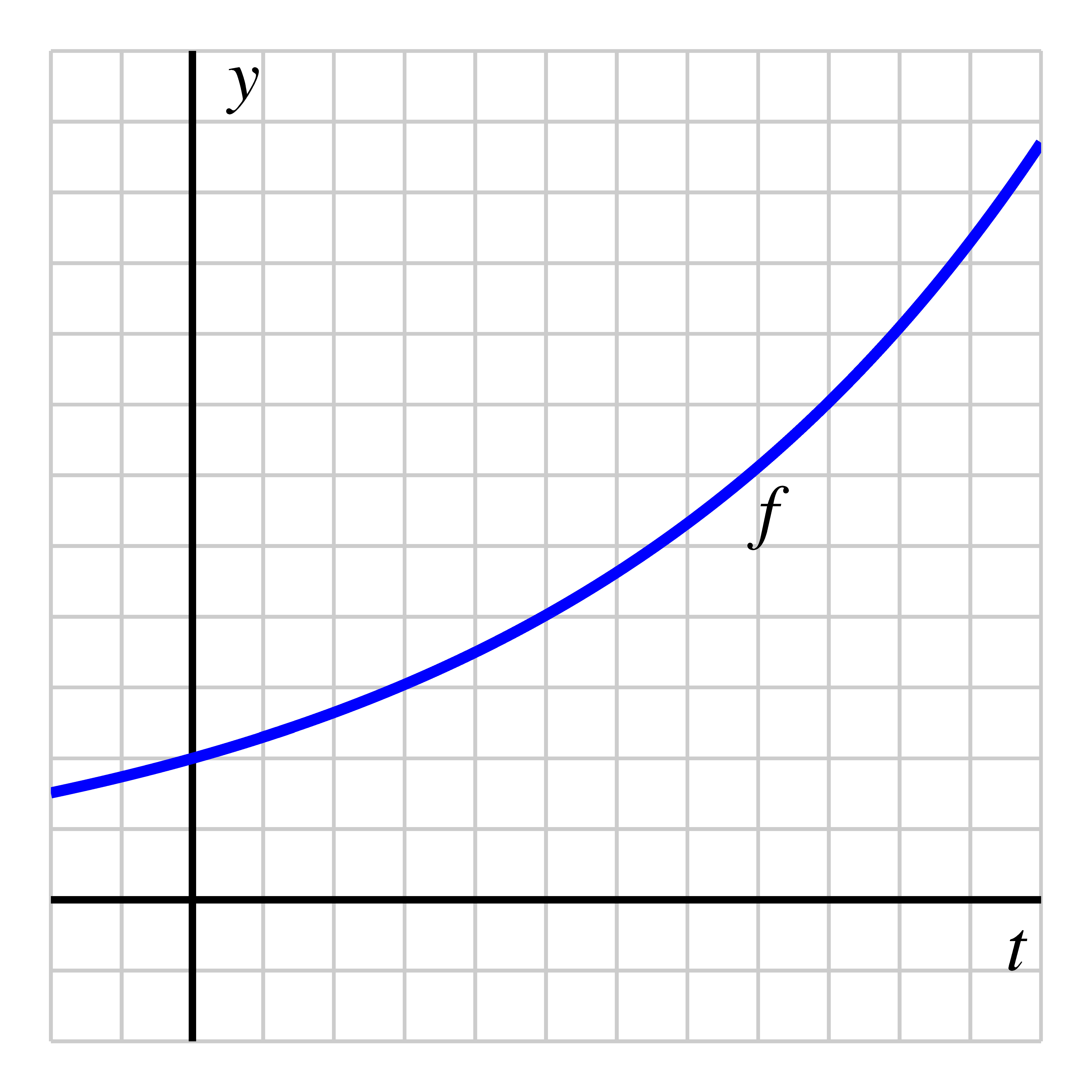
If we consider an exponential function with a growth factor , such as the function
pictured in the left-hand graph above, then the function is always increasing because
higher powers of are greater than lesser powers (for example, ). On the other hand, if
, then the exponential function will be decreasing because higher powers of positive
numbers less than get smaller (e.g., ), as seen for the exponential function in the
right-hand graph above.
An additional trend is apparent in the graphs in above. Each graph bends upward
and is therefore concave up. We can better understand why this is so by
considering the average rate of change of both and on consecutive intervals of the
same width. We choose adjacent intervals of length and note particularly
that as we compute the average rate of change of each function on such
intervals,
Thus, these average rates of change are also measuring the total change in the
function across an interval that is -unit wide. We now assume that and
and compute the rate of change of each function on several consecutive
intervals.
The average rate of change of
The average rate of change of
From the data in the first table about we see that the average rate of change is
increasing as we increase the value of . We naturally say that appears to be
“increasing at an increasing rate”. For the function , we first notice that its average
rate of change is always negative, but also that the average rate of change gets less
negative as we increase the value of . Said differently, the average rate of change of is
also increasing as we increase the value of . Since is always decreasing but its average
rate of change is increasing, we say that appears to be “decreasing at an increasing
rate”. These trends hold for exponential functions generally according to
the conditions given below. It takes calculus to justify this claim fully and
rigorously.
Trends in exponential function behavior.
For an exponential function of the form where and are both positive with
,
if , then is always increasing and always increases at an increasing rate;
if , then is always decreasing and always decreases at an increasing rate.
If a function is always increasing and always increases at an increasing rate, it is
concave up, and vice-versa. If a function is always decreasing and always decreases at
an increasing rate, it is concave down, and vice-versa.
Observe how a function’s average rate of change helps us classify the function’s
behavior on an interval: whether the average rate of change is always positive or
always negative on the interval enables us to say if the function is always increasing
or always decreasing, and then how the average rate of change itself changes enables
us to potentially say how the function is increasing or decreasing through phrases
such as “decreasing at an increasing rate”.
For each of the following prompts, give an example of a function that satisfies the
stated characteristics by both providing a formula and sketching a graph.
a.
A function that is always decreasing and decreases at a constant rate.
b.
A function that is always increasing and increases at an increasing rate.
c.
A function that is always increasing for , always decreasing for , and is
always changing at a decreasing rate.
d.
A function that is always increasing and increases at a decreasing rate.
(Hint: to find a formula, think about how you might use a transformation
of a familiar function.)
e.
A function that is always decreasing and decreases at a decreasing rate.
We say that a function is exponential whenever its algebraic form is for
some positive constants and where . (Technically, the formal definition
of an exponential function is one of form , but in our everyday usage of
the term “exponential” we include vertical stretches of these functions and
thus allow to be any positive constant, not just .)
To determine the formula for an exponential function of form , we need to know
two pieces of information. Typically this information is presented in one of two
ways.
If we know the amount, , of a quantity at time and the rate, , at
which the quantity grows or decays per unit time, then it follows .
In this setting, is often given as a percentage that we convert to a
decimal (e.g., if the quantity grows at a rate of % per year, we set ,
so ).
If we know any two points on the exponential function’s graph, then
we can set up a system of two equations in two unknowns and solve
for both and exactly. In this situation, it is useful to consider the
quotient of the two known outputs, as demonstrated in Example example:exp1.
Exponential functions of the form (where and are both positive and ) exhibit
the following important characteristics:
The domain of any exponential function is the set of all real numbers
and the range of any exponential function is the set of all positive
real numbers.
The -intercept of the exponential function is and the function has
no -intercepts.
If , then the exponential function is always increasing and always
increases at an increasing rate. If , then the exponential function is
always decreasing and always decreases at an increasing rate.