- a.
- Set and explore the effects of changing the values of and . Write several sentences to summarize your observations.
- b.
- Follow the directions for (a) again, this time with
- c.
- Set and . Explore the effects of changing the value of ; be sure to include values of both less than and greater than 1. Write several sentences to summarize your observations.
- d.
- When , what happens to the graph of when we consider positive -values that get larger and larger?
Motivating Questions
- What can we say about the behavior of an exponential function as the input gets larger and larger?
- How do vertical stretches and shifts of an exponontial function affect its behavior?
- Why is the temperature of a cooling or warming object modeled by a function of the form ?
Introduction
If a quantity changes so that its growth or decay occurs at a constant percentage rate with respect to time, the function is exponential. This is because if the growth or decay rate is , the total amount of the quantity at time is given by , where is the amount present at time . Many different natural quantities change according to exponential models: money growth through compounding interest, the growth of a population of cells, and the decay of radioactive elements
A related situation arises when an object’s temperature changes in response to its surroundings. For instance, if we have a cup of coffee at an initial temperature of Fahrenheit and the cup is placed in a room where the surrounding temperature is , our intuition and experience tell us that over time the coffee will cool and eventually tend to the temperature of the surroundings. From an experiment with an actual temperature probe, we have the data in the table below.
Data for cooling coffee
(measured in degrees Fahrenheit at the time t in minutes)
Here is a graph of these points.
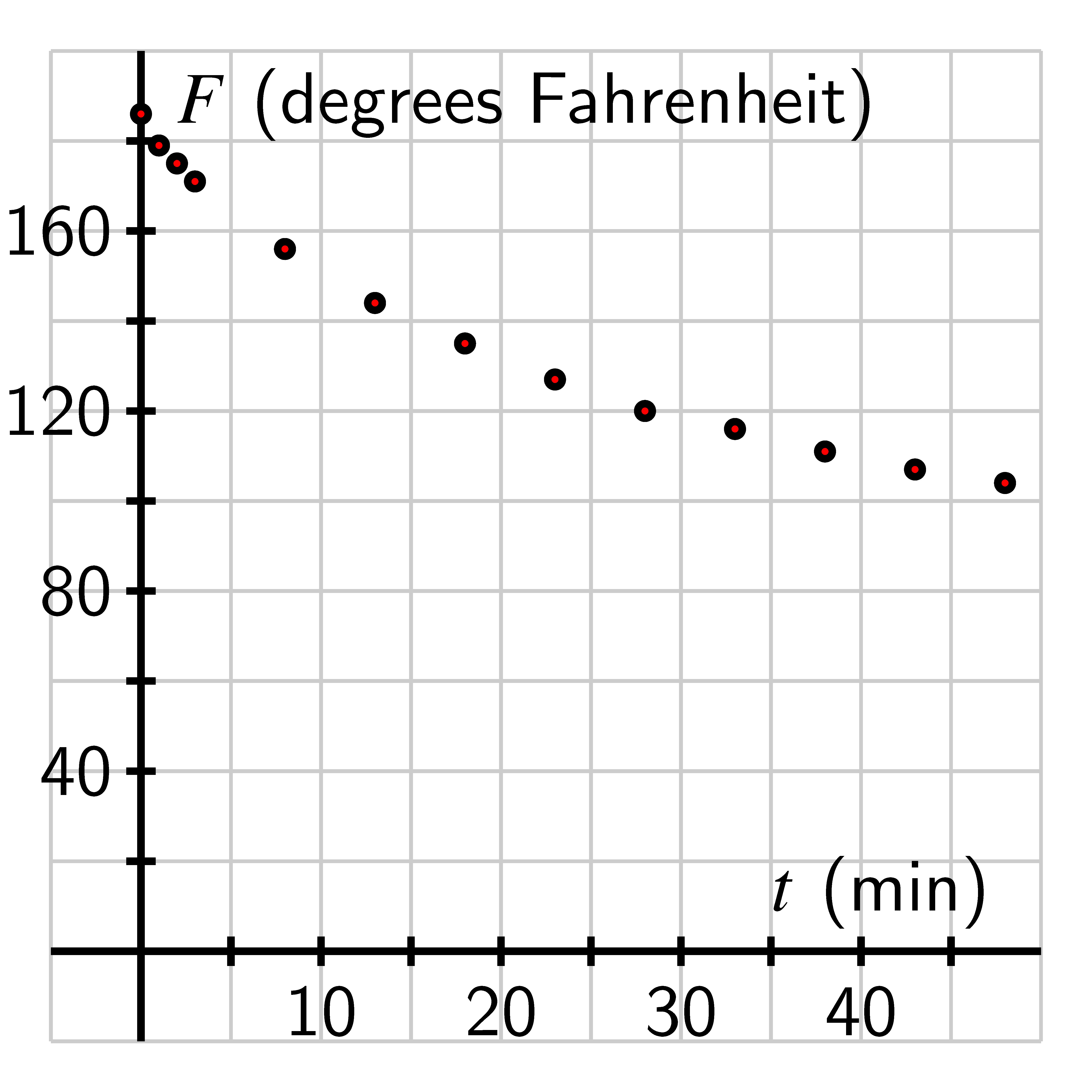
In one sense, the data looks exponential: the points appear to lie on a curve that is always decreasing and decreasing at an increasing rate. However, we know that the function can’t have the form because such a function’s range is the set of all positive real numbers, and it’s impossible for the coffee’s temperature to fall below room temperature (). It is natural to wonder if a function of the form will work. Thus, in order to find a function that fits the data in a situation such as this, we begin by investigating and understanding the roles of , , and in the behavior of .
In Desmos, define and accept the prompt for sliders for , , and . Edit the sliders so
that has values from to , has values from to , and has values from to (also with a
step-size of 0.01). In addition, in Desmos let and check the box to show the
label. Finally, zoom out so that the window shows an interval of -values from
End behavior of exponential functions
We have already established that any exponential function of the form where and are positive real numbers with is always concave up and is either always increasing or always decreasing. We next introduce precise language to describe the behavior of an exponential function’s value as gets bigger and bigger. To start, let’s consider the two basic exponential functions and and their respective values at , , and , as displayed below.
For the increasing function , we see that the output of the function gets very large very quickly. In addition, there is no upper bound to how large the function can be. Indeed, we can make the value of as large as we’d like by taking sufficiently big. We thus say that as increases, increases without bound.
For the decreasing function , we see that the output is always positive but getting closer and closer to . Indeed, becasue we can make as large as we like, it follows that we can make its reciprocal as small as we’d like. We thus say that as increases, approaches .
To represent these two common phenomena with exponential functions the value increasing without bound or the value approaching , we will use shorthand notation. First, it is natural to write “” as increases without bound. Moreover, since we have the notion of the infinite to represent quantities without bound, we use the symbol for infinity () and write “” as increases without bound in order to indicate that increases without bound.
In the exploration above, we saw how the value of affects the steepness of the graph of , as well as how all graphs with have the similar increasing behavior, and all graphs with have similar decreasing behavior. For instance, by taking sufficiently large, we can make as large as we want; it just takes much larger to make big in comparison to . In the same way, we can make as close to as we wish by taking sufficiently big, even though it takes longer for to get close to in comparison to . For an arbitrary choice of , we can say the following.
End behavior of exponential functions. Let with and
.
- If , then as . We read this notation as “ tends to as increases without bound.” Also, as . We read this notation as “ increases without bound as decreases without bound.”
- If , then as . We read this notation as “ increases without bound as increases without bound.” Also, as . We read this notation as “ tends to as decreases without bound.”
In addition, we make a key observation about the use of exponents. For the function , there are three equivalent ways we may write the function:
In our work with transformations involving horizontal scaling, we saw that the graph of is the reflection of the graph of across the -axis. Therefore, we can say that the graphs of and are reflections of one another across the -axis since . We see this fact verified in the graph below.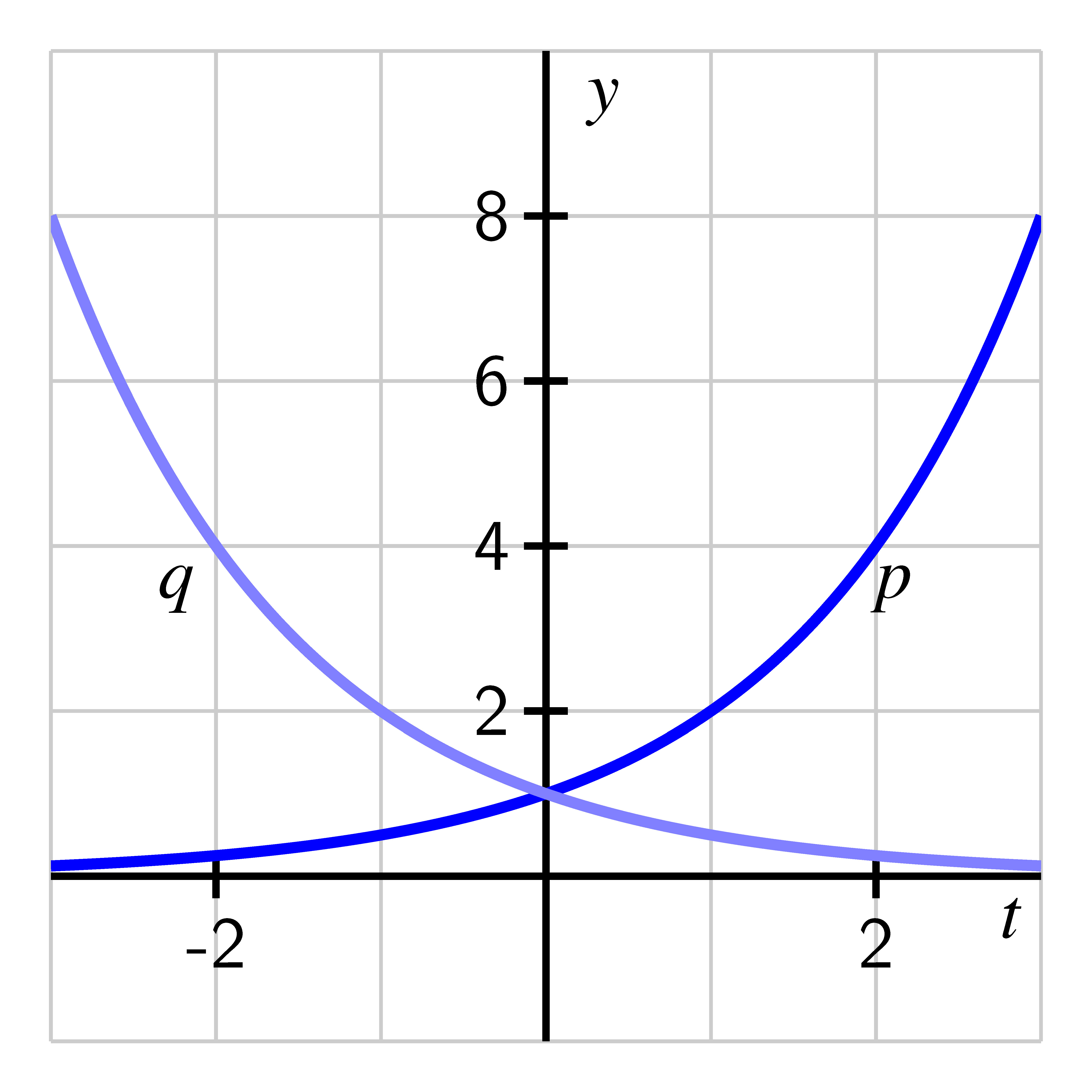
Similar observations hold for the relationship between the graphs of and for any positive .
- If the base of an exponential function satisfies , as and as .
- If the base of an exponential function satisfies , as and as .
The role of in
The function is a vertical translation of the function . We now have extensive understanding of the behavior of and how that behavior depends on and . Since a vertical translation by does not change the shape of any graph, we expect that will exhibit very similar behavior to . Indeed, we can compare the two functions’ graphs as shown in the graphs belowA and then make the following general observations.
Behavior of vertically shifted exponential functions.
Let with , and , and any real number.
- If , then as . The function is always decreasing, always concave up, and has -intercept . The range of the function is all real numbers greater than .
- If , then as . The function is always increasing, always concave up, and has -intercept . The range of the function is all real numbers greater than .
It is also possible to have . In this situation, because is both a reflection of across the -axis and a vertical stretch by , the function is always concave down. If so that is always decreasing, then is always increasing; if instead so is increasing, then is decreasing. Moreover, instead of the range of the function having a lower bound as when , in this setting the range of has an upper bound. These ideas are explored further below.
It’s an important skill to be able to look at an exponential function of the form and form an accurate mental picture of the graph’s main features in light of the values of , , and .
For each of the following functions, without using graphing technology, determine
whether the function is
- i.
- always increasing or always decreasing;
- ii.
- always concave up or always concave down; and
- iii.
- increasing without bound, decreasing without bound, or increasing/decreasing toward a finite value.
In addition, state the -intercept and the range of the function. For each function, write a sentence that explains your thinking and sketch a rough graph of how the function appears.
- a.
- b.
- c.
- d.
- e.
- f.
Modeling temperature data
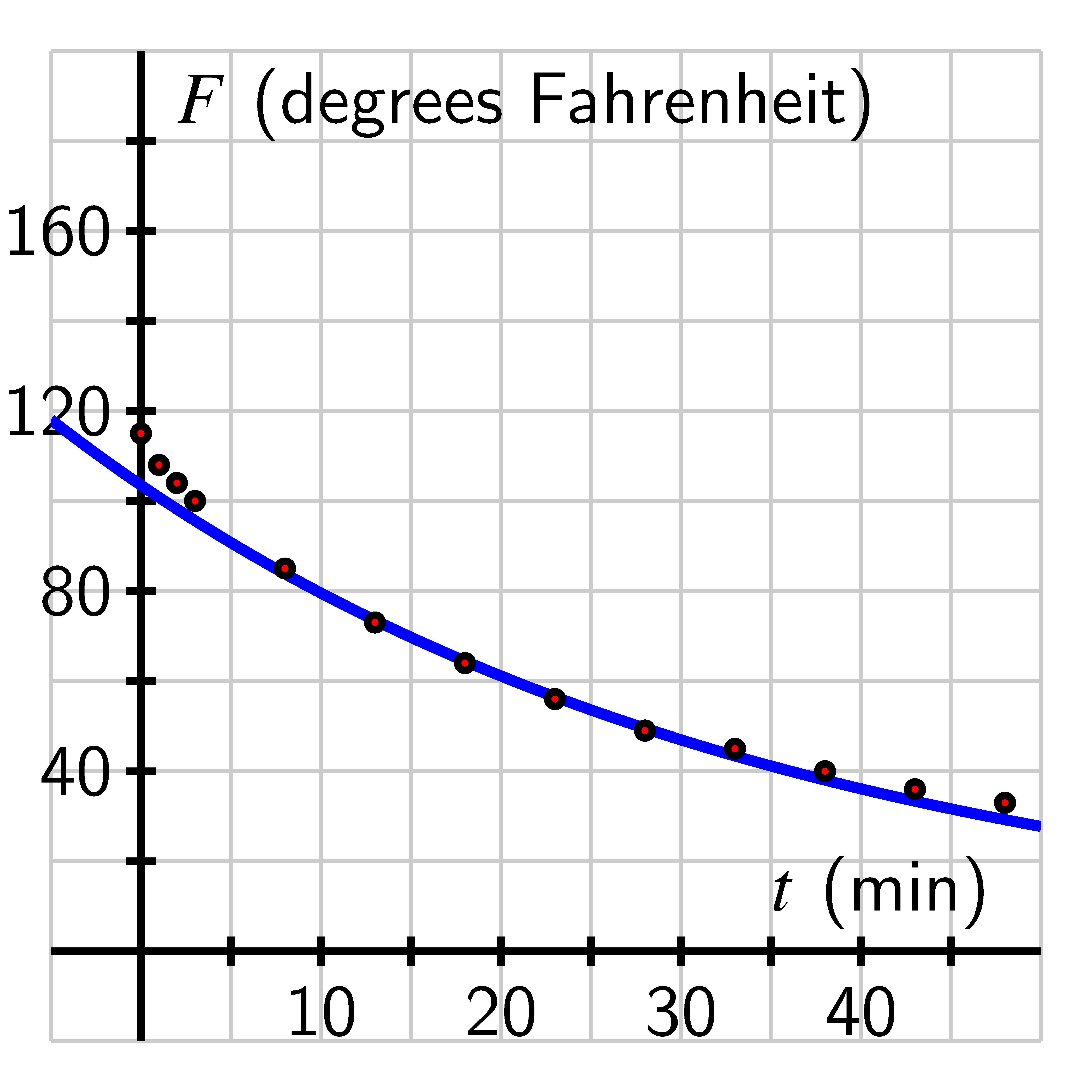
Newton’s Law of Cooling states that the rate that an object warms or cools occurs in direct proportion to the difference between its own temperature and the temperature of its surroundings. If we return to the coffee temperature data and recall that the room temperature in that experiment was , we can see how to use a transformed exponential function to model the data. In the table below, we add a row of information to the table where we compute to subtract the room temperature from each reading.
Data for cooling coffee
(measured in degrees Fahrenheit at the time t in minutes)
The data in the last row of the table appears exponential, and if we test the data by computing the quotients of output values that correspond to equally-spaced input, we see a nearly constant ratio. In particular,
Of course there is some measurement error in the data (plus it is only recorded to accuracy of whole degrees), so these computations provide convincing evidence that the underlying function is exponential. In addition, we expect that if the data continued in the last of the table, the values would approach because will approach .If we choose two of the data points, say and , and assume that , we can determine the values of and . Since the above points are on the graph, we know that and , that is, and . Solving for in both equations, we find that and . Equating these expressions tells us that , and cross-multiplying gives us . Cancelling gives us , or . Now we can plug this into our earlier expression for to find that .
Using a calculator, we can see that and , so . We’ll use the name to refer to the approximate function . Since , we see that , so . We’ll use the name to refer to the approximate function . Plotting against the shifted data and along with the original data in the graphs above, we see that the curves go exactly through the points where and as expected, but also that the function provides a reasonable model for the observed behavior at any time . If our data was even more accurate, we would expect that the curve’s fit would be even better.
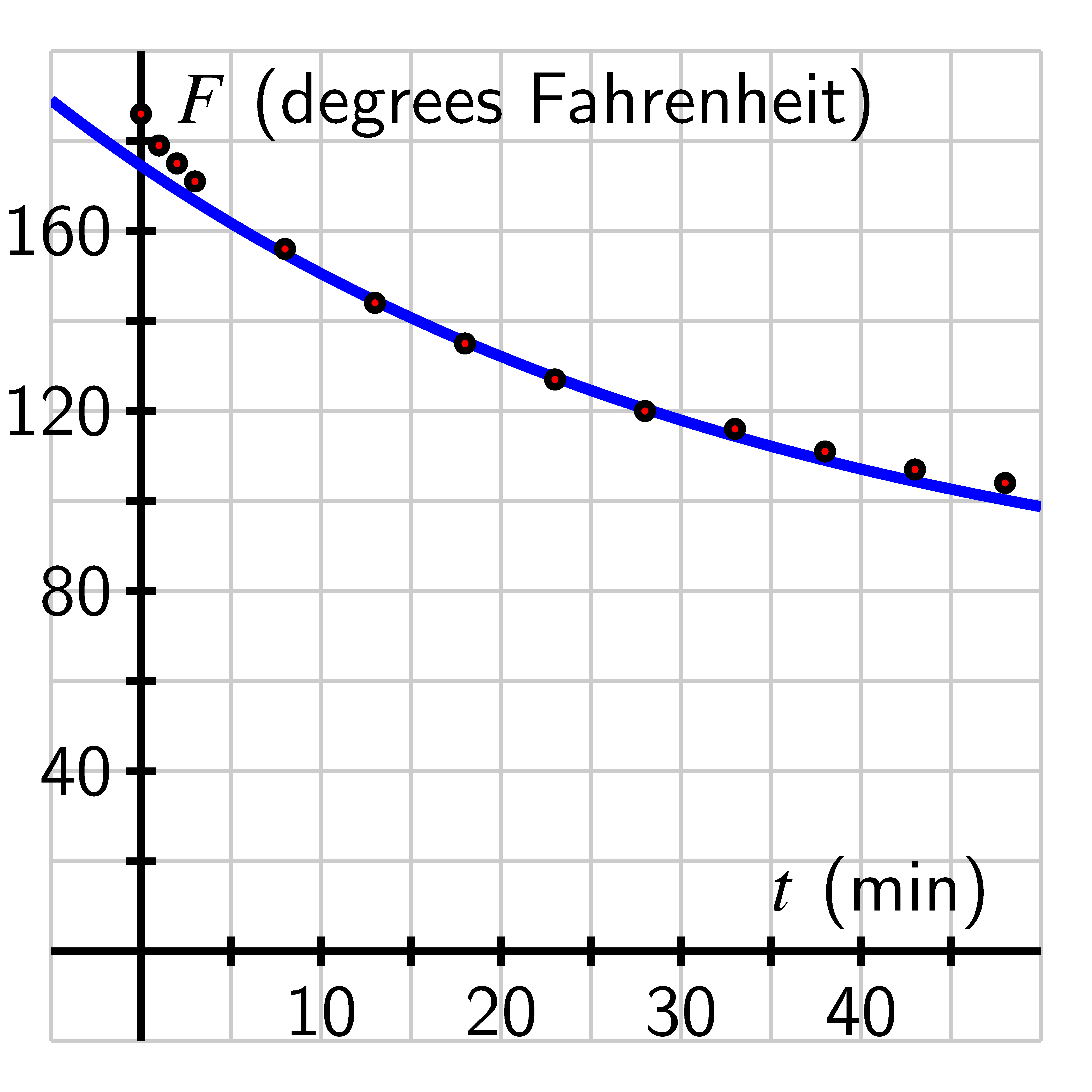
Our preceding work with the coffee data can be done similarly with data for any cooling or warming object whose temperature initially differs from its surroundings. Indeed, it is possible to show that Newton’s Law of Cooling implies that the object’s temperature is given by a function of the form .
A can of soda (at room temperature) is placed in a refrigerator at time (in minutes)
and its temperature, , in degrees Fahrenheit, is computed at regular intervals. Based
on the data, a model is formulated for the object’s temperature, given by
- a.
- Consider the simpler (parent) function . How do you expect the graph of this function to appear? How will it behave as time increases? Without using graphing technology, sketch a rough graph of and write a sentence of explanation.
- b.
- For the slightly more complicated function , how do you expect this function to look in comparison to ? What is the long-range behavior of this function as increases? Without using graphing technology, sketch a rough graph of and write a sentence of explanation.
- c.
- Finally, how do you expect the graph of to appear? Why? First sketch a rough
graph without graphing technology, and then use technology to check your
thinking and report an accurate, labeled graph on the axes provided.
- d.
- What is the temperature of the refrigerator? What is the room temperature of the surroundings outside the refrigerator? Why?
- e.
- Determine the average rate of change of on the intervals , , and . Write at least two careful sentences that explain the meaning of the values you found, including units, and discuss any overall trend in how the average rate of change is changing.
A potato initially at room temperature () is placed in an oven (at ) at time . It is
known that the potato’s temperature at time is given by the function for some
positive constants and , where is measured in degrees Fahrenheit and is time in
minutes.
- a.
- What is the numerical value of ? What does this tell you about the value of ?
- b.
- Based on the context of the problem, what should be the long-range behavior of the function ? Use this fact along with the behavior of to determine the value of . Write a sentence to explain your thinking.
- c.
- What is the value of ? Why?
- d.
- Check your work above by plotting the function using graphing technology in
an appropriate window. Record your results on the axes provided, labeling the
scale on the axes. Then, use the graph to estimate the time at which the
potato’s temperature reaches degrees.
- e.
- How can we view the function as a transformation of the parent function ? Explain.
- For an exponential function of the form , the function either approaches zero or grows without bound as the input gets larger and larger. In particular, if , then as , while if , then as . Scaling by a positive value (that is, the transformed function ) does not affect the long-range behavior: whether the function tends to or increases without bound depends solely on whether is less than or greater than .
- The function passes through , is always concave up, is either always increasing or always decreasing, and its range is the set of all positive real numbers. Among these properties, a vertical stretch by a positive value only affects the -intercept, which is instead . If we include a vertical shift and write , the biggest changes is that the range of is the set of all real numbers greater than . In addition, the -intercept of is .
- In the situation where , several other changes are induced. Here, because is both a reflection of across the -axis and a vertical stretch by , the function is now always concave down. If so that is always decreasing, then (the reflected function) is now always increasing; if instead so is increasing, then is decreasing. Finally, if , then the range of is the set of all real numbers .
- An exponential function can be thought of as a function that changes at a rate proportional to itself, like how money grows with compound interest or the amount of a radioactive quantity decays. Newton’s Law of Cooling says that the rate of change of an object’s temperature is proportional to the difference between its own temperature and the temperature of its surroundings. This leads to the function that measures the difference between the object’s temperature and room temperature being exponential, and hence the object’s temperature itself is a vertically-shifted exponential function of the form .