Coupled Linear Systems

$\newenvironment {prompt}{}{} \newcommand {\Sec }[2]{\section {#1}} \newcommand {\trademark }[0]{{R\!\!\!\!\!\bigcirc }} \newcommand {\EXER }[0]{\section *{Exercises}} \newcommand {\CEXER }[0]{} \newcommand {\TEXER }[0]{} \newcommand {\R }[0]{\mbox {$\Bbb {R}$}} \newcommand {\C }[0]{\mbox {$\Bbb {C}$}} \newcommand {\Z }[0]{\mbox {$\Bbb {Z}$}} \newcommand {\N }[0]{\mbox {$\Bbb {N}$}} \newcommand {\D }[0]{\mbox {{\bf D}}} \newcommand {\setmin }[0]{\;\mbox {--}\;} \newcommand {\Matlab }[0]{{M\small {AT\-LAB}} } \newcommand {\Matlabp }[0]{{M\small {AT\-LAB}}} \newcommand {\computer }[0]{\Matlab Instructions} \newcommand {\half }[0]{\mbox {$\frac {1}{2}$}} \newcommand {\compose }[0]{\raisebox {.15ex}{\mbox {{\scriptsize $\circ $}}}} \newcommand {\AND }[0]{\quad \mbox {and}\quad } \newcommand {\vect }[2]{\left (\begin {array}{c} #1_1 \\ \vdots \\ #1_{#2}\end {array}\right )} \newcommand {\mattwo }[4]{\left (\begin {array}{rr} #1 & #2\\ #3 &#4\end {array}\right )} \newcommand {\mattwoc }[4]{\left (\begin {array}{cc} #1 & #2\\ #3 &#4\end {array}\right )} \newcommand {\vectwo }[2]{\left (\begin {array}{r} #1 \\ #2\end {array}\right )} \newcommand {\vectwoc }[2]{\left (\begin {array}{c} #1 \\ #2\end {array}\right )} \newcommand {\inv }[0]{^{-1}} \newcommand {\CC }[0]{{\cal C}} \newcommand {\CCone }[0]{\CC ^1} \newcommand {\Span }[0]{{\rm span}} \newcommand {\rank }[0]{{\rm rank}} \newcommand {\trace }[0]{{\rm tr}} \newcommand {\RE }[0]{{\rm Re}} \newcommand {\IM }[0]{{\rm Im}} \newcommand {\nulls }[0]{{\rm null\;space}} \newcommand {\dps }[0]{\displaystyle } \newcommand {\arraystart }[0]{\renewcommand {\arraystretch }{1.8}} \newcommand {\arrayfinish }[0]{\renewcommand {\arraystretch }{1.2}} \newcommand {\Start }[1]{\vspace {0.08in}\noindent {\bf Section~\ref {#1}}} \newcommand {\exer }[1]{\noindent {\bf \ref {#1}}} \newcommand {\ans }[0]{} \newcommand {\matthree }[9]{\left (\begin {array}{rrr} #1 & #2 & #3 \\ #4 & #5 & #6 \\ #7 & #8 & #9\end {array}\right )} \newcommand {\cvectwo }[2]{\left (\begin {array}{c} #1 \\ #2\end {array}\right )} \newcommand {\cmatthree }[9]{\left (\begin {array}{ccc} #1 & #2 & #3 \\ #4 & #5 & #6 \\ #7 & #8 & #9\end {array}\right )} \newcommand {\vecthree }[3]{\left (\begin {array}{r} #1 \\ #2 \\ #3\end {array}\right )} \newcommand {\cvecthree }[3]{\left (\begin {array}{c} #1 \\ #2 \\ #3\end {array}\right )} \newcommand {\cmattwo }[4]{\left (\begin {array}{cc} #1 & #2\\ #3 &#4\end {array}\right )} \newcommand {\thehelp }[0]{\thesection .\arabic {equation}} \newcommand {\matlabEquation }[0]{\let \oldtheequation \theequation \renewcommand {\theequation }{\oldtheequation *}\begin {equation}} \newcommand {\HyperFirstAtBeginDocument }[0]{\AtBeginDocument } \newcommand {\epstopdfsetup }[0]{\setkeys {ETE}} changed the theorem header of amsthm failed\MessageBreak }}} \newcommand {\GetTitleStringSetup }[0]{\setkeys {gettitlestring}} \newcommand {\Sectionformat }[2]{#1} \newcommand {\arraystretch }[0]{1.8} \newcommand {\arraystretch }[0]{1.0}$ $% This file was *autogenerated* from coupledLinearSystems.sagetex.sage with % sagetex.py version 2015/08/26 v3.0-92d9f7a %f67fd6f1bf9a9e6b7bb0c827ce947aec% md5sum of corresponding .sage file (minus "goboom","current_tex_line",and pause/unpause lines)$

The general linear constant coefficient system in two unknown functions $x_1,x_2$ is:

$\begin{equation} \label{lin3} \begin{array}{ccc} \dps \frac{dx_1}{dt}(t) & = & ax_1(t) + bx_2(t) \\ \dps \frac{dx_2}{dt}(t) & = & cx_1(t) + dx_2(t). \end{array} \end{equation}$ The uncoupled systems studied in Section ?? are obtained by setting $b=c=0$ in (??). We have discussed how to solve (??) by formula (??) when the system is uncoupled. We have also discussed how to visualize the phase plane for different choices of the diagonal entries $a$ and $d$ . At present, we cannot solve (??) by formula when the coefficient matrix is not diagonal. But we may use pplane5 to solve the initial value problems numerically for these coupled systems. We illustrate this point by solving

$\begin{eqnarray*} \frac{dx_1}{dt}(t) & = & -x_1(t) + 3x_2(t) \\ \frac{dx_2}{dt}(t) & = & 3x_1(t) - x_2(t). \end{eqnarray*}$

After starting pplane5, select linear system from the Gallery and set the constants to: $a = -1,\quad b = 3,\quad c = 3, \quad d = -1.$ Click on Proceed. In order to have equally spaced coordinates on the $x$ and $y$ axes, do the following. In the PPLANE5 Display window click on the edit button and then on the zoom in square command. Then, using the mouse, click on the origin.

Eigendirections

After computing several solutions, we find that for increasing time $t$ all the solutions seem to approach the diagonal line given by the equation $x_1=x_2$ . Similarly, in backward time $t$ the solutions approach the anti-diagonal $x_1=-x_2$ . In other words, as for the case of uncoupled systems, we find two distinguished directions in the $(x,y)$ -plane. See Figure ??. Moreover, the computations indicate that these lines are invariant in the sense that solutions starting on these lines remain on them for all time. This statement can be verified numerically by using the Keyboard input in the PPLANE5 Options to choose initial conditions $(x_0,y_0)=(1,1)$ and $(x_0,y_0)=(1,-1)$ .

Figure 1: PPLANE5 Display for (??) with $a=-1=d$ ; $b=3=c$ ; and $x,y\in [-5,5]$ . Solutions going through $(\pm 0.5,0)$ and $(0,\pm 0.5)$ are shown.

An invariant line for a linear system of differential equations is called an eigendirection.

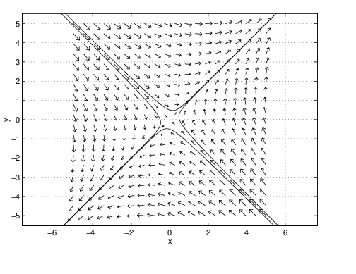
Observe that eigendirections vary if we change parameters. For example, if we set $b$ to $1$ , then there are still two distinguished lines but these lines are no longer perpendicular.

For uncoupled systems, we have shown analytically that the $x$ and $y$ axes are eigendirections. The numerical computations that we have just performed indicate that eigendirections exist for many coupled systems. This discussion leads naturally to two questions:

(a): Do eigendirections always exist?
(b): How can we find eigendirections?

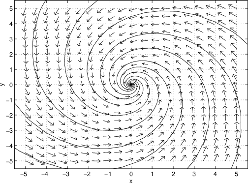
The second question will be answered in Sections ?? and ??. We can answer the first question by performing another numerical computation. In the setup window, change the parameter $b$ to $-2$ . Then numerically compute some solutions to see that there are no eigendirections in the phase space of this system. Observe that all solutions appear to spiral into the origin as time goes to infinity. The phase portrait is shown in Figure ??.

Figure 2: PPLANE5 Display for the linear system with $a=-1$ , $b=-2$ , $c=3$ , $d=-1$ .

Second Order Differential Equations

We now show analytically that certain linear systems of differential equations have no invariant lines in their phase portrait.

We do this by showing that second order differential equations can be reduced to first order systems by a simple but important trick. Indeed, sometimes it is easier to solve a single second order equation, and sometimes it is easier to solve the first order system. At this stage we introduce this connection by considering the differential equation

$\begin{equation} \label{E:2ndordera} \frac{d^2x}{dt^2} + x = 0. \end{equation}$ This differential equation states that we are looking for a function $x(t)$ whose second derivative is $-x(t)$ . From calculus, we know that $x(t)=\cos t$ is such a function.

Let $y(t)=\dot {x}(t)$ . Then (??) may be rewritten as a first order coupled system in $x(t)$ and $y(t)$ as follows:

$\begin{equation} \label{E:2nd->1st} \begin{array}{rcl} \dot{x} & = & y \\ \dot{y} & = & -x. \end{array} \end{equation}$ Observe that if $x(t)$ is a solution to (??), then $0 = \frac {d^2x}{dt^2} + x = \frac {dy}{dt} + x.$ Hence, $\dot {y} = -x$ Conversely, if $(x(t),y(t))$ is a solution to (??), then $x(t)$ is a solution to (??). That is, $\frac {d^2x}{dt^2} + x = \frac {dy}{dt} + x = -x + x = 0.$

It follows from the discussion that $(x(t),y(t))=(\cos t,\sin t)$ is a solution to the differential equation (??). We have shown analytically that the unit circle centered at the origin is a solution trajectory for (??). Hence (??) has no eigendirections. It may be checked using MATLAB that all solution trajectories for (??) are just circles centered at the origin.

Exercises

Choose the linear system in pplane5 and set $a=0$ , $b=1$ , and $c=-1$ . Then find values $d$ such that except for the origin itself all solutions appear to

spiral into the origin;
spiral away from the origin;
form circles around the origin;

Choose the linear system in pplane5 and set $a=-1$ , $c=3$ , and $d=-1$ . Then find a value for $b$ such that the behavior of the solutions of the system is “qualitatively” the same as for a diagonal system where $a$ and $d$ are negative. In particular, the origin should be an asymptotically stable equilibrium and the solutions should approach that equilibrium along a distinguished line.

Choose the linear system in pplane5 and set $a=d$ and $b=c$ . Verify that for these systems of differential equations:

When $|a|<b$ typical trajectories approach the line $y=x$ as $t\to \infty$ and the line $y=-x$ as $t\to -\infty$ .
Assume that $b$ is positive, $a$ is negative, and $b<-a$ . With these assumptions show that the origin is a sink and that typical trajectories approach the origin tangent to the line $y=x$ .

Sketch the time series $y(t)$ for the solution to the differential equation whose phase plane is pictured in Figure ?? with initial condition $(x(0),y(0))=(\frac {1}{2},\frac {1}{2})$ . Check your answer using pplane5.

In Exercises ?? – ??, determine which of the function pairs $(x_1(t),y_1(t))$ and $(x_2(t),y_2(t))$ are solutions to the given system of ordinary differential equations.

The ODE is:

$\begin{eqnarray*} \dot{x} & = & 2x+y \\ \dot{y} & = & 3y. \end{eqnarray*}$

The pairs of functions are: $(x_1(t),y_1(t)) = (e^{2t},0) \AND (x_2(t),y_2(t)) = (e^{3t},e^{3t}).$

The ODE is:

$\begin{eqnarray*} \dot{x} & = & 2x - 3y \\ \dot{y} & = & x - 2y. \end{eqnarray*}$

The pairs of functions are: $(x_1(t),y_1(t)) = e^t(3,1) \AND (x_2(t),y_2(t)) = (e^{-t},e^{-t}).$

The ODE is:

$\begin{eqnarray*} \dot{x} & = & x + y \\ \dot{y} & = & -x + y. \end{eqnarray*}$

The pairs of functions are: $(x_1(t),y_1(t)) = (3e^t, -2e^t) \AND (x_2(t),y_2(t)) = e^t(\sin t,\cos t).$

The ODE is:

$\begin{eqnarray*} \dot{x} & = & y \\ \dot{y} & = & -\frac{1}{t^2}x + \frac{1}{t}y + 1. \end{eqnarray*}$

The pairs of functions are: $(x_1(t),y_1(t)) = (t^2,2t) \AND (x_2(t),y_2(t)) = (2t^2,4t).$