The Continuous Flow Stirred Tank Reactor

$\newenvironment {prompt}{}{} \newcommand {\Sec }[2]{\section {#1}} \newcommand {\trademark }[0]{{R\!\!\!\!\!\bigcirc }} \newcommand {\EXER }[0]{\section *{Exercises}} \newcommand {\CEXER }[0]{} \newcommand {\TEXER }[0]{} \newcommand {\R }[0]{\mbox {$\Bbb {R}$}} \newcommand {\C }[0]{\mbox {$\Bbb {C}$}} \newcommand {\Z }[0]{\mbox {$\Bbb {Z}$}} \newcommand {\N }[0]{\mbox {$\Bbb {N}$}} \newcommand {\D }[0]{\mbox {{\bf D}}} \newcommand {\setmin }[0]{\;\mbox {--}\;} \newcommand {\Matlab }[0]{{M\small {AT\-LAB}} } \newcommand {\Matlabp }[0]{{M\small {AT\-LAB}}} \newcommand {\computer }[0]{\Matlab Instructions} \newcommand {\half }[0]{\mbox {$\frac {1}{2}$}} \newcommand {\compose }[0]{\raisebox {.15ex}{\mbox {{\scriptsize $\circ $}}}} \newcommand {\AND }[0]{\quad \mbox {and}\quad } \newcommand {\vect }[2]{\left (\begin {array}{c} #1_1 \\ \vdots \\ #1_{#2}\end {array}\right )} \newcommand {\mattwo }[4]{\left (\begin {array}{rr} #1 & #2\\ #3 &#4\end {array}\right )} \newcommand {\mattwoc }[4]{\left (\begin {array}{cc} #1 & #2\\ #3 &#4\end {array}\right )} \newcommand {\vectwo }[2]{\left (\begin {array}{r} #1 \\ #2\end {array}\right )} \newcommand {\vectwoc }[2]{\left (\begin {array}{c} #1 \\ #2\end {array}\right )} \newcommand {\inv }[0]{^{-1}} \newcommand {\CC }[0]{{\cal C}} \newcommand {\CCone }[0]{\CC ^1} \newcommand {\Span }[0]{{\rm span}} \newcommand {\rank }[0]{{\rm rank}} \newcommand {\trace }[0]{{\rm tr}} \newcommand {\RE }[0]{{\rm Re}} \newcommand {\IM }[0]{{\rm Im}} \newcommand {\nulls }[0]{{\rm null\;space}} \newcommand {\dps }[0]{\displaystyle } \newcommand {\arraystart }[0]{\renewcommand {\arraystretch }{1.8}} \newcommand {\arrayfinish }[0]{\renewcommand {\arraystretch }{1.2}} \newcommand {\Start }[1]{\vspace {0.08in}\noindent {\bf Section~\ref {#1}}} \newcommand {\exer }[1]{\noindent {\bf \ref {#1}}} \newcommand {\ans }[0]{} \newcommand {\matthree }[9]{\left (\begin {array}{rrr} #1 & #2 & #3 \\ #4 & #5 & #6 \\ #7 & #8 & #9\end {array}\right )} \newcommand {\cvectwo }[2]{\left (\begin {array}{c} #1 \\ #2\end {array}\right )} \newcommand {\cmatthree }[9]{\left (\begin {array}{ccc} #1 & #2 & #3 \\ #4 & #5 & #6 \\ #7 & #8 & #9\end {array}\right )} \newcommand {\vecthree }[3]{\left (\begin {array}{r} #1 \\ #2 \\ #3\end {array}\right )} \newcommand {\cvecthree }[3]{\left (\begin {array}{c} #1 \\ #2 \\ #3\end {array}\right )} \newcommand {\cmattwo }[4]{\left (\begin {array}{cc} #1 & #2\\ #3 &#4\end {array}\right )} \newcommand {\thehelp }[0]{\thesection .\arabic {equation}} \newcommand {\matlabEquation }[0]{\let \oldtheequation \theequation \renewcommand {\theequation }{\oldtheequation *}\begin {equation}} \newcommand {\HyperFirstAtBeginDocument }[0]{\AtBeginDocument } \newcommand {\epstopdfsetup }[0]{\setkeys {ETE}} changed the theorem header of amsthm failed\MessageBreak }}} \newcommand {\GetTitleStringSetup }[0]{\setkeys {gettitlestring}} \newcommand {\Sectionformat }[2]{#1} \newcommand {\arraystretch }[0]{1.8} \newcommand {\arraystretch }[0]{1.2} \newcommand {\theequation }[0]{\oldtheequation *}$ $% This file was *autogenerated* from theContinuousFlowStirredTankReactor.sagetex.sage with % sagetex.py version 2015/08/26 v3.0-92d9f7a %088080486bd8b73e0335c2c5e0015e92% md5sum of corresponding .sage file (minus "goboom","current_tex_line",and pause/unpause lines)$

Perhaps the simplest chemical engineering model of a chemical reaction is the CSTR — the continuous flow stirred tank chemical reactor. In the CSTR we imagine that a reactant flows into a vessel and undergoes a single heat producing reaction to form inert products. The concentration of the reactant inside the vessel is denoted by $c$ and the temperature of the fluid inside the vessel is denoted by $T$ . The assumption that the tank is well stirred is interpreted mathematically to mean that $c$ and $T$ are constant everywhere in the vessel. The CSTR model describes how $c$ and $T$ evolve in time.

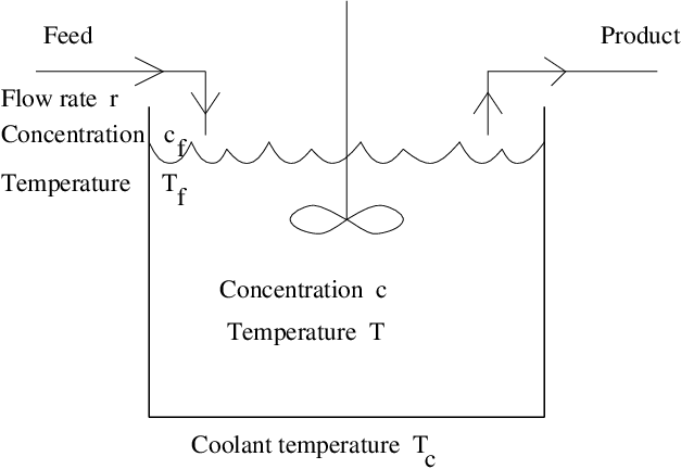
The CSTR is pictured schematically in Figure ??. We assume that the reactant flows into a unit volume vessel at a constant rate $r$ and that the product flows out of the vessel at the same rate. The fluid that flows into the vessel is called the feed. We assume that the temperature of the feed is held constant at $T_f$ and that the reactant concentration of the feed is $c_f$ . We also assume that the vessel is surrounded by a coolant whose temperature $T_c$ is held constant.

Figure 1: Schematic diagram for CSTR.

The Reactionless CSTR

Ignoring the effects of the chemical reaction, the model equations describing the time evolution of the temperature and concentration of the reactant in the vessel are:

$\begin{equation} \label{e:CSTRlin} \begin{array}{rcl} \dps\frac{dc}{dt} & = & r(c_f-c) \\ \dps\frac{dT}{dt} & = & r(T_f-T) + k(T_c-T), \end{array} \end{equation}$ where $k$ is a lumped parameter that depends on a variety of physical quantities including heat transfer area and specific heat.

So far, the model in (??) is an inhomogeneous uncoupled system of linear differential equations. We have assumed that the concentration of the reactant grows exponentially to the feed concentration at rate $r$ . The fate of the temperature inside the vessel is less clear, as we have assumed that the temperature grows exponentially to the feed temperature at rate $r$ and simultaneously grows exponentially to the coolant temperature at rate $k$ (that is just Newton’s law of cooling). At this point, we have not modeled the effects of the chemical reaction on concentration and temperature inside the vessel — though we have modeled how the external variables such as feed temperature and concentration and the coolant temperature affect the concentration and temperature inside the vessel. For this reason, this model is called the reactionless CSTR. Before continuing with the modeling, we nondimensionalize the variables, as engineers prefer to do.

In this model, we have assumed implicitly that concentration and temperature are positive quantities. For concentration this is clearly a reasonable assumption. For temperature this means that we are measuring temperature from absolute zero. Suppose that we let $x(t) = \frac {c(\frac {t}{k})-c_f}{c_f} \AND y(t) = \frac {T(\frac {t}{k})-T_f}{T_f}$ be scaled concentration and temperature. We have normalized $x$ and $y$ to measure deviation from the feed concentration and temperature, and we have scaled $c$ and $T$ by $c_f$ and $T_f$ so that the state variables $x$ and $y$ are nondimensional — they have no physical units attached to them. In addition, we have scaled time by the lumped rate constant $k$ . (Chemical engineers do not usually scale time in the equations, since $k$ is a parameter that can be controlled in experiments.) Next, let $\eta = \frac {T_c-T_f}{T_f} \AND \rho = \frac {r}{k}$ be the nondimensionalized coolant temperature and flow rate, respectively. Note that the fact that all physical quantities were assumed to be positive leads to the restrictions $x, y,\eta >-1 \AND \rho >0.$

Observe that $\frac {dx}{dt}(t)=\frac {1}{kc_f}\frac {dc}{dt}\left (\frac {t}{k}\right ) \AND \frac {dy}{dt}(t)=\frac {1}{kT_f}\frac {dT}{dt}\left (\frac {t}{k}\right ).$ Coupling this observation with (??) yields the equations for the reactionless CSTR in nondimensionalized form:

$\begin{eqnarray} \dot{x} & = & -\rho x \label{e:ndCSTRlina} \\ \dot{y} & = & -(\rho+1)y + \eta. \label{e:ndCSTRlinb} \end{eqnarray}$

The solution to (??) is $x(t) = e^{-\rho t}x_0,$ and, in the absence of a reaction, the scaled concentration decays exponentially to $x=0$ , that is, to the feed concentration.

The solution to (??) is slightly more complicated to obtain in closed form, as this is an example of an inhomogeneous linear equation. Using superposition, we can find the general solution to the inhomogeneous equation by finding one solution to the inhomogeneous equation and adding in all solutions to the homogeneous equation. In this case, it is easy to find a constant solution to the inhomogeneous equation. Just set

$\begin{equation} \label{e:basetemp} y = \frac{\eta}{\rho+1}, \end{equation}$ and check that this constant is a solution to (??). As we know, $y(t) = e^{-(\rho +1)t}K$ is the general solution to the homogeneous equation, and $y(t) = e^{-(\rho +1)t}K + \frac {\eta }{\rho +1}$ is the general solution to (??). Thus, temperature decays exponentially to (??), the coolant temperature in nondimensionalized form scaled by the nondimensionalized flow rate.

The CSTR

Next we consider the effects of the reaction. For thermodynamic reasons, which we do not discuss here, we assume that the reaction depletes the reactant at a temperature dependent rate proportional to concentration times the Arrhenius term $A(y)$ where $A(y) = \exp \left (\frac {\gamma y}{y+1}\right )$ and $\gamma$ is the activation energy. Since the reaction is heat producing, we also assume that the temperature of the reactant increases at a rate proportional to $cA(y)$ . Since the concentration $c$ is proportional to $x+1$ , these assumptions lead to the nonlinear system of differential equations

$\begin{equation} \label{e:CSTR} \begin{array}{rcl} \dot{x} & = & -\rho x - Z(x+1)A(y) \\ \dot{y} & = & -(\rho+1)y + \eta + hZ(x+1)A(y), \end{array} \end{matlabEquation} where $Z$ and $h$ are proportionality constants. In this form the equations have two state variables $x,y$ and five constants $\rho,\eta,\gamma,Z,h$. (The CSTR equation in {\tt e12\_3\_5.pps} has $\gamma=4$ so that there are just four parameters.) \subsection*{Numerical Solution of the CSTR} \index{CSTR} It is a difficult problem to determine the phase portraits for the CSTR equations for all values of the five constants. Here we use {\sf pplane5} to indicate some of the different phase portraits that can occur in these equations. In order to simplify the task, we fix values for all parameters except the nondimensionalized flow rate $\rho$. We set \begin{equation} \label{e:CSTRparam} \gamma=4, \quad \eta=-0.75, \quad Z=0.5, \quad h =3. 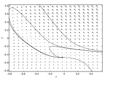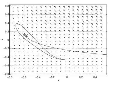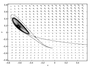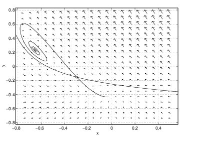\end{equation}$ Numerical experimentation on the rectangle $-0.75\leq x \leq 0.5$ , $-0.75\leq y\leq 0.75$ shows the following. There are three possible equilibria — one at high temperature ( $y\sim 0.1$ ), one at medium temperature ( $y\sim -0.1$ ), and one at low temperature ( $y\sim -0.5$ ). For these parameter values, the equilibrium at medium temperature is always a saddle and the equilibrium at low temperature is always a sink. We present the phase portraits for five values of the nondimensionalized flow rate $\rho$ . The results are as follows:

The only equilibrium is the low temperature equilibrium and it is a nodal sink.
There are three equilibria. The high temperature spiral source and the medium temperature saddle appear as $\rho$ is increased. Note that the stable orbit of the saddle connects directly to the spiral source.
The high temperature equilibrium is a spiral sink and the stable orbit of the saddle connects to a limit cycle. At this parameter value, there are two stable equilibria.
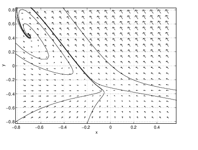
There are still three equilibria, but the time-periodic solution has disappeared. The unstable orbit of the saddle now connects to the high temperature spiral sink. The low temperature sink is a spiral sink and there are two stable spiral sinks.
The only remaining equilibrium is the high temperature spiral sink. The saddle and the low temperature sink have coalesced and disappeared. (Presumably the low temperature spiral sink became a nodal sink before it coalesced with the saddle.)

These calculations show that the phase portrait of the CSTR changes between successive values of $\rho$ , that is, we have shown that there are at least four bifurcation values in the CSTR as $\rho$ is varied. The five different phase planes are shown in Figure ??.

$\hspace {1.2in} \mbox {$\rho =0.495$ \hspace {2.0in} $\rho =0.52$}$

$\hspace {1.2in} \mbox {$\rho =0.545$ \hspace {2.0in} $\rho =0.57$}$

$\rho =0.72$

Figure 2: Phase portraits of CSTR (??) with $\gamma =4$ , $\eta =-0.75$ , $Z=0.5$ , $h =3$ .

Bifurcations in the CSTR

The observed bifurcations in the CSTR divide into local and global bifurcations, as we now discuss.

As we saw in Section ??, local bifurcations are of two types: steady-state (saddle-node) and Hopf. For example, in Figure ??, we see that as the parameter $\rho$ is decreased from $0.52$ to $0.495$ the middle and high temperature equilibria collide and disappear at a saddle-node bifurcation. See Exercise ?? for further verification of this fact. Similarly, between the values of $\rho =0.57$ and $\rho =0.72$ the low and middle temperature equilibria collide and disappear. We presume that a saddle-node bifurcation has also occurred in this parameter regime.

A different bifurcation occurs as $\rho$ increases from $0.52$ and $0.545$ . In this range, the high temperature spiral changes from a source to a sink. For this change to occur, there must be a parameter value where the high temperature equilibrium is a center. Since a time periodic solution is found in the phase portrait of the CSTR at $\rho =0.545$ , we conclude that a Hopf bifurcation has occurred in this parameter region.

Both of these local bifurcations occur at parameter values where there is a nonhyperbolic equilibrium. As we noted, Hopf bifurcation occurs at a parameter value where a center is present, while steady-state bifurcation occurs at a parameter value where an equilibrium has a Jacobian matrix with a zero eigenvalue — typically a saddle-node.

A global bifurcation, one in which the bifurcation in phase portraits occurs away from equilibria, is present in the CSTR between $\rho =0.545$ and $\rho =0.57$ . In this region, the periodic solution grows until it touches the saddle point. At that point, one branch of the stable orbit and one branch of the unstable orbit of the saddle are identical. Thus, there is a trajectory that limits on the saddle point in both forward and backward time. As we saw in Section ?? such trajectories are called homoclinic trajectories and such bifurcations are called homoclinic bifurcations. Note the similarity between the phase portraits in Figure ?? and the middle phase portraits in Figure ??.

There are other global bifurcations that we have not seen in these equations. Two periodic solutions can collide and both disappear (just like the saddle-node steady-state bifurcation where two equilibria collide and disappear). This bifurcation is discussed in Section ??. Another global bifurcation occurs when the stable orbit of one saddle point coincides with the unstable orbit of another saddle point. This bifurcation is called a saddle-saddle connection. The homoclinic bifurcation is a special case of a saddle-saddle connection where the two saddle points are the same. See Section ??.

Bifurcation Diagrams

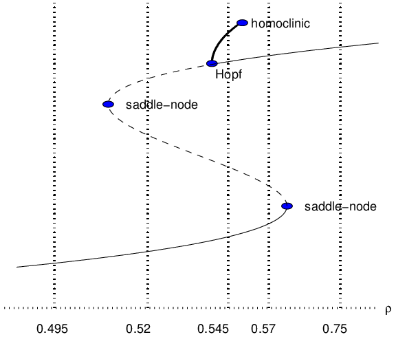
The discussion of transitions in the CSTR can be summarized by the use of a bifurcation diagram, as introduced in Section ??. In a bifurcation diagram we graph the equilibria and periodic solutions of equations as a function of the parameter $\rho$ . In bifurcation diagrams:

A saddle-node bifurcation appears as a turning point in a branch of equilibria.
A Hopf bifurcation appears as a change in stability along a branch of equilibria.
A homoclinic bifurcation is noted by a sudden ending of a branch of periodic solutions.

In the CSTR equations we have numerical evidence for two saddle-node bifurcations, a Hopf bifurcation, and a homoclinic bifurcation. This information is illustrated in the bifurcation diagram in Figure ??. Bifurcation diagrams contain an enormous amount of information — and it takes practice to learn to read them. For example, suppose $\rho$ is fixed to be $0.545$ in Figure ??. Then we may surmise that there are three equilibria of the CSTR equations at that value of $\rho$ — the low and high temperature equilibria are asymptotically stable while the middle temperature one is not — and an unstable limit cycle (that surrounds the high temperature equilibrium).

Figure 3: Schematic bifurcation diagram for the CSTR

Exercises

Consider the CSTR equations (??) with parameters (??). Set $\rho =0.5$ and use pplane5 to verify that there are two equilibria — a low temperature nodal sink and a middle temperature saddle-node equilibrium. Then change $\rho$ to $0.505$ and verify that the saddle-node has split into two equilibria — a saddle and a spiral source.

Use pplane5 to explore the CSTR equations (??) with parameters: $h=2, \quad Z=0.5, \quad \eta =-0.5, \quad \gamma =5,$ for various values of the parameter $\rho$ between $0.46$ and $0.51$ . Describe all equilibria and all periodic solutions that you find, and how they change as $\rho$ is varied.