Saddle-Node Bifurcations Revisited

$\newenvironment {prompt}{}{} \newcommand {\Sec }[2]{\section {#1}} \newcommand {\trademark }[0]{{R\!\!\!\!\!\bigcirc }} \newcommand {\EXER }[0]{\section *{Exercises}} \newcommand {\CEXER }[0]{} \newcommand {\TEXER }[0]{} \newcommand {\R }[0]{\mbox {$\Bbb {R}$}} \newcommand {\C }[0]{\mbox {$\Bbb {C}$}} \newcommand {\Z }[0]{\mbox {$\Bbb {Z}$}} \newcommand {\N }[0]{\mbox {$\Bbb {N}$}} \newcommand {\D }[0]{\mbox {{\bf D}}} \newcommand {\setmin }[0]{\;\mbox {--}\;} \newcommand {\Matlab }[0]{{M\small {AT\-LAB}} } \newcommand {\Matlabp }[0]{{M\small {AT\-LAB}}} \newcommand {\computer }[0]{\Matlab Instructions} \newcommand {\half }[0]{\mbox {$\frac {1}{2}$}} \newcommand {\compose }[0]{\raisebox {.15ex}{\mbox {{\scriptsize $\circ $}}}} \newcommand {\AND }[0]{\quad \mbox {and}\quad } \newcommand {\vect }[2]{\left (\begin {array}{c} #1_1 \\ \vdots \\ #1_{#2}\end {array}\right )} \newcommand {\mattwo }[4]{\left (\begin {array}{rr} #1 & #2\\ #3 &#4\end {array}\right )} \newcommand {\mattwoc }[4]{\left (\begin {array}{cc} #1 & #2\\ #3 &#4\end {array}\right )} \newcommand {\vectwo }[2]{\left (\begin {array}{r} #1 \\ #2\end {array}\right )} \newcommand {\vectwoc }[2]{\left (\begin {array}{c} #1 \\ #2\end {array}\right )} \newcommand {\inv }[0]{^{-1}} \newcommand {\CC }[0]{{\cal C}} \newcommand {\CCone }[0]{\CC ^1} \newcommand {\Span }[0]{{\rm span}} \newcommand {\rank }[0]{{\rm rank}} \newcommand {\trace }[0]{{\rm tr}} \newcommand {\RE }[0]{{\rm Re}} \newcommand {\IM }[0]{{\rm Im}} \newcommand {\nulls }[0]{{\rm null\;space}} \newcommand {\dps }[0]{\displaystyle } \newcommand {\arraystart }[0]{\renewcommand {\arraystretch }{1.8}} \newcommand {\arrayfinish }[0]{\renewcommand {\arraystretch }{1.2}} \newcommand {\Start }[1]{\vspace {0.08in}\noindent {\bf Section~\ref {#1}}} \newcommand {\exer }[1]{\noindent {\bf \ref {#1}}} \newcommand {\ans }[0]{} \newcommand {\matthree }[9]{\left (\begin {array}{rrr} #1 & #2 & #3 \\ #4 & #5 & #6 \\ #7 & #8 & #9\end {array}\right )} \newcommand {\cvectwo }[2]{\left (\begin {array}{c} #1 \\ #2\end {array}\right )} \newcommand {\cmatthree }[9]{\left (\begin {array}{ccc} #1 & #2 & #3 \\ #4 & #5 & #6 \\ #7 & #8 & #9\end {array}\right )} \newcommand {\vecthree }[3]{\left (\begin {array}{r} #1 \\ #2 \\ #3\end {array}\right )} \newcommand {\cvecthree }[3]{\left (\begin {array}{c} #1 \\ #2 \\ #3\end {array}\right )} \newcommand {\cmattwo }[4]{\left (\begin {array}{cc} #1 & #2\\ #3 &#4\end {array}\right )} \newcommand {\thehelp }[0]{\thesection .\arabic {equation}} \newcommand {\matlabEquation }[0]{\let \oldtheequation \theequation \renewcommand {\theequation }{\oldtheequation *}\begin {equation}} \newcommand {\HyperFirstAtBeginDocument }[0]{\AtBeginDocument } \newcommand {\epstopdfsetup }[0]{\setkeys {ETE}} changed the theorem header of amsthm failed\MessageBreak }}} \newcommand {\GetTitleStringSetup }[0]{\setkeys {gettitlestring}} \newcommand {\Sectionformat }[2]{#1} \newcommand {\theequation }[0]{\oldtheequation *}$ $% This file was *autogenerated* from saddleNodeBifurcationsRevisited.sagetex.sage with % sagetex.py version 2015/08/26 v3.0-92d9f7a %74395201e20e5654b7a15fa2e7467805% md5sum of corresponding .sage file (minus "goboom","current_tex_line",and pause/unpause lines)$

The simplest steady-state bifurcations — and the ones that are most likely to occur — are the saddle-node bifurcations. In Section ?? we found necessary conditions for the existence of saddle-node bifurcations in one dimension (??) and two dimensions (??). In this section we describe necessary and sufficient conditions for the existence of saddle-node bifurcations.

Saddle-Node Bifurcation in One Dimension

Consider the differential equation

$\begin{equation} \label{e:1dbif} \dot{x} = f(x,\rho), \end{equation}$ that depends on the single parameter $\rho$ . The equilibria are found by solving the algebraic equation $\begin{equation} \label{e:1dstst} f(x,\rho) = 0. \end{equation}$ We can study how the equilibria in phase portraits for (??) change when $\rho$ is varied by plotting solutions to (??) in the $\rho x$ -plane. The solutions to (??) form the bifurcation diagram of (??).

Recall from (??) that

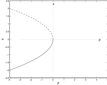
$\begin{equation} \label{e:1dbifcond} \begin{array}{rcl} f(x_0,\rho_0) & = & 0 \\ f_x(x_0,\rho_0) & = & 0. \end{array} \end{equation}$ are necessary conditions for a saddle-node bifurcation to occur at $(x_0,\rho _0)$ . The simplest example of a saddle-node bifurcation is: $\begin{equation} \label{e:1dsaddlenf} f(x,\rho) = a x^2 + \rho, \end{equation}$ where $a$ is a nonzero constant. The exact bifurcation diagram for (??) depends on the sign of $a$ . See Figure ??. Note that the bifurcation diagram is just a parabola pointing either to the left or to the right. The general saddle-node bifurcation is one whose bifurcation diagram looks ‘parabolic-like’. Theorem ?? makes this idea precise.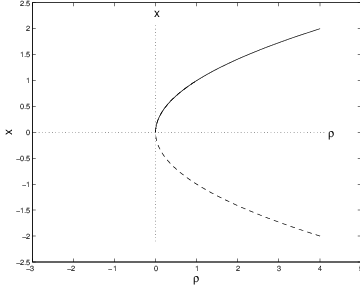

$a<0$ $a>0$

Figure 1: Bifurcation diagrams for (??).

Suppose that the differential equation (??) has an equilibrium at $(x_0,\rho _0)$ satisfying the bifurcation conditions (??) and the nondegeneracy conditions $\begin{equation} \label{e:nondegen1} \begin{array}{rcl} f_\rho(x_0,\rho_0) & \neq & 0 \\ f_{xx}(x_0,\rho_0) & \neq & 0. \end{array} \end{equation}$ Then the bifurcation diagram $f=0$ looks like the diagram in Figure ?? where $a = \frac {f_{xx}(x_0,\rho _0)}{f_\rho (x_0,\rho _0)}.$

Proof

The proof of this theorem uses the implicit function theorem and implicit differentiation. (Technically, we need to assume that the second derivatives of $f(x,\rho )$ are continuous before proceeding.) Since $f_\rho (x_0,\rho _0)$ is assumed to be nonzero, the implicit function theorem guarantees the existence of a function $R(x)$ such that $R(x_0)=\rho _0$ and $\begin{equation} \label{e:implicit0} f(x,R(x))\equiv 0 \end{equation}$ for all $x$ near $x_0$ . It follows that the bifurcation diagram $f(x,\rho )=0$ is the graph $\rho = R(x)$ . We claim that $R'(x_0)=0$ and $R''(x_0)\neq 0$ . Thus the Taylor series of the function $R(x)$ is $R(x) = \rho _0 + \half R''(x_0)(x-x_0)^2 + \cdots$ for all $x$ near $x_0$ . It follows that the bifurcation diagram $f=0$ is parabolic in shape as in Figure ?? — opening either to the left or to the right depending on the sign of $R''(x_0)$ .

We use implicit differentiation to verify these claims. Differentiating (??) twice yields

$\begin{equation} \label{e:implicit1} f_x(x,R(x)) + f_\rho(x,R(x))R'(x) \equiv 0, \end{equation}$ and $\begin{equation} \label{e:implicit2} f_{xx}(x,R(x)) + 2f_{x\rho}(x,R(x))R'(x) + f_{\rho\rho}(x,R(x))R'(x)^2 + f_\rho(x,R(x))R''(x) \equiv 0. \end{equation}$

Evaluating (??) at $x=x_0$ yields $f_x(x_0,\rho _0) + f_\rho (x_0,\rho _0)R'(x_0) = 0.$ Since, by assumption, $f_x(x_0,\rho _0)=0$ and $f_\rho (x_0,\rho _0)\neq 0$ , it follows that $R'(x_0)=0.$ Evaluating (??) at $x=x_0$ now yields $f_{xx}(x_0,\rho _0) + f_\rho (x_0,\rho _0)R''(x_0) = 0$ The nondegeneracy assumptions (??) imply $R''(x_0) = -\frac {f_{xx}(x_0,\rho _0)}{f_\rho (x_0,\rho _0)} \neq 0.$ Thus $a=-R''(x_0)$ . So when $R''(x_0)>0$ the number $a$ is negative and the bifurcating branch is supercritical, as in Figure ??. Similarly, when $R''(x_0)<0$ the number $a$ is positive and the bifurcating branch is subcritical. $\blacksquare$

An Example of a One Dimensional Saddle-Node Bifurcation

Consider the following example of a saddle-node bifurcation. Let

$\begin{equation} \label{e:sn1} f(x,\rho) = -x^3 + 3x^2 - \rho x - 4. \end{equation}$ A quick check shows that $x=2$ is an equilibrium for (??) when $\rho =0$ . Moreover, $f(2,0)=0, \quad f_x(2,0)=0, \quad f_\rho (2,0)=-2\neq 0, \quad f_{xx}(2,0)=-6\neq 0.$ It follows from Theorem ?? that $f$ has a saddle-node bifurcation when $\rho =0$ at $x=2$ . Indeed, since $a=\frac {-6}{-2}=3>0$ , it follows that there are two equilibria near $x=2$ when $\rho <0$ and none when $\rho >0$ . See Figure ??. This fact can be verified using pline. When $\rho$ is small and positive, there is one stable equilibrium near $x=-1$ . When $\rho$ is small and negative, there are three equilibria — the stable one near $x=-1$ and two new equilibria near $x=2$ formed from the saddle-node bifurcation.

Saddle-Node Bifurcations in Two Dimensions

In higher dimensions, steady-state bifurcations occur at parameter values where the Jacobian matrix has a zero eigenvalue. In one dimension, the $1\times 1$ Jacobian matrix is the number $f_x$ . Such a Jacobian matrix has a zero eigenvalue precisely when $f_x$ vanishes — which is just the condition in (??).

In two dimensions, the Jacobian matrix $J$ is a saddle-node matrix when it has a single zero eigenvalue, that is, when $\det (J)=0$ and $\trace (J)\neq 0$ . Now consider the planar system of differential equations depending on a parameter $\rho$ . We write this system as

$\begin{equation} \label{e:2deqn} \dot{X} = F(X,\rho), \end{equation}$ where $X=(x,y)\in \R ^2$ and $F=(g,h)$ in coordinates. Sufficient conditions for the existence of a saddle-node bifurcation in (??) are as follows.

(a): Equation (??) has an equilibrium at $(X_0,\rho _0)$ ; so $F(X_0,\rho _0) = 0.$
(b): The Jacobian matrix $J=(dF)_{(X_0,\rho _0)}= \mattwo {g_x(X_0,\rho _0)}{g_y(X_0,\rho _0)}{h_x(X_0,\rho _0)}{h_y(X_0,\rho _0)}.$ has a zero eigenvalue and a nonzero eigenvalue. Let $w$ be a nonzero vector in the null space of $J^t$ . Assume $\begin{equation} \label{e:2deig} w \cdot F_\rho(X_0,\rho_0) \neq 0, \end{equation}$ where $F_\rho =(g_\rho ,h_\rho )$ . (In one dimension, (??) just states that $f_\rho (X_0,\rho _0)$ is nonzero; that is, the first nondegeneracy condition in (??) is valid.)
(c): Let $v=(v_1,v_2)$ be a nonzero vector in the null space of $J$ . The following is an analogue in two dimensions for the second nondegeneracy condition in (??), $f_{xx}(x_0,\rho _0)\neq 0$ . Define $F_0$ to be the vector $F_0 = v_1^2\vectwo {g_{xx}}{h_{xx}} + 2v_1v_2\vectwo {g_{xy}}{h_{xy}} + v_2^2 \vectwo {g_{yy}}{h_{yy}}$ evaluated at $(X_0,\rho _0)$ . The nondegeneracy condition in two dimensions is: $\begin{equation} \label{e:2dbifur} w \cdot F_0 \neq 0. \end{equation}$

A steady-state bifurcation is a saddle-node bifurcation if (??) and (??) are valid. At a saddle-node bifurcation two equilibria coalesce as $\rho$ is varied, and the bifurcation diagram resembles that in Figure ??.

An Example of a Two Dimensional Saddle-Node Bifurcation

As an example, consider the system of differential equations

$\begin{equation} \label{e:snex} \begin{array}{rcccl} \dot{x} & = & \rho + x + 3y -xy & \equiv & g(x,y) \\ \dot{y} & = & -\rho + 2x + 6y + 3x^2 & \equiv & h(x,y). \end{array} \end{matlabEquation} At $\rho = 0$, \eqref{e:snex} has an equilibrium at the origin with Jacobian matrix \[ J = \mattwo{1}{3}{2}{6}. \] Since $\det(J)=0$, the origin is a bifurcation point. Define the vectors $v$ and $w$ by \[ Jv=0 \AND J^tw=0. \] So \[ v = \vectwo{3}{-1} \AND w = \vectwo{2}{-1}. \] Next compute \[ F_\rho = \vectwo{1}{-1}. \] Therefore \[ w \cdot F_\rho = \vectwo{2}{-1} \cdot \vectwo{1}{-1} = 3 \neq 0, \] and \eqref{e:2deig} is satisfied. Next compute \[ g_{xx}=0, \quad g_{xy}=-1, \quad g_{yy}=0, \quad h_{xx}=6, \quad h_{xy}=0, \quad h_{yy} = 0. \] Hence \[ F_0 = v_1^2 \vectwo{0}{6} + 2v_1v_2\vectwo{-1}{0} = \vectwo{6}{54}, \] and \[ w\cdot F_0 = \vectwo{2}{-1} \cdot \vectwo{6}{54} = -42 \neq 0. \] So \eqref{e:2dbifur} is satisfied. These conditions show that there is a saddle-node bifurcation at the origin and that two equilibria coalesce as $\rho$ varies through zero. Some experimentation will convince you that it is complicated to find a closed form analytic solution for the equilibria of \eqref{e:snex}. We can, however, verify the existence of a saddle-node bifurcation using {\sf pplane5}. The phase plane portraits are shown in Figure~\ref{F:snex}. \begin{figure}[htb] \centerline{% \psfig{file=../figures/snexa.eps,width=3.2in} \psfig{file=../figures/snexb.eps,width=3.2in}} \vspace*{-0.2in} \hspace{1.0in} $\rho=-0.1$ \hspace{2.55in} $\rho=0.1$ \caption{Phase plane portrait for \protect\eqref{e:snex} on the square $-1\leq x,y \leq 1$. Note that there are no equilibria when $\rho=-0.1$ and two equilibria when $\rho=0.1$.} \label{F:snex} \end{figure} \EXER \TEXER \begin{exercise} \label{c9.3.1} Let \begin{eqnarray*} f_1(x,\rho) & = & \rho - x^3 \\ f_2(x,\rho) & = & \rho x - x^2. \end{eqnarray*} \begin{itemize} \item[(a)] Verify that both $f_1$ and $f_2$ satisfy the bifurcation conditions \eqref{e:1dbifcond} at $x=0$ when $\rho=0$. \item[(b)] Show that neither $f_1$ nor $f_2$ has a saddle-node bifurcation at $x=0$ when $\rho=0$. \item[(c)] Draw the bifurcation diagrams $f_1(x,\rho)=0$ and $f_2(x,\rho)=0$ and explain why the conclusion of Theorem~\ref{T:saddlenode} is not satisfied for either $f_1$ or $f_2$. \end{itemize} \end{exercise} \begin{exercise} \label{c9.3.5} Find all saddle-node bifurcations in the family of differential equations \begin{equation} \dot{x} = x^3 -5x^2 + 3x + \rho \end{equation}$ analytically. Draw the bifurcation diagram.

Let $f(x,\rho ) = x^4 - 6x^3 +8x^2 + 6(x-\rho ) - 3.$ Show that $f$ has a saddle-node bifurcation at $x=3$ when $\rho =1$ . Are there two equilibria near $x=3$ when $\rho <1$ or when $\rho >1$ ?

Let

$\begin{eqnarray*} g(x,y,\rho) & = & \rho - 2x + y + 2x^2 - y^3 \\ h(x,y,\rho) & = & 2\rho + 4x - 2y - xy + y^2 \end{eqnarray*}$

Show that $F=(g,h)$ has a saddle-node bifurcation at $(x,y)=0$ and $\rho =0$ .

Let $X=(x,y)$ and $F(X,\rho ) = \rho q + \mattwo {1}{0}{0}{0} X + Q(X)$ where $q=\vectwo {q_1}{q_2} \AND Q(X) = \vectwo {\alpha x^2+\beta xy+\gamma y^2} {\delta x^2 +\epsilon xy+\varphi y^2}.$ Show that $F$ has a saddle-node bifurcation at $X=0$ and $\rho =0$ precisely when $q_2\neq 0$ and $\varphi \neq 0$ .