Nonconstant Coefficient Linear Equations

$\newenvironment {prompt}{}{} \newcommand {\Sec }[2]{\section {#1}} \newcommand {\trademark }[0]{{R\!\!\!\!\!\bigcirc }} \newcommand {\EXER }[0]{\section *{Exercises}} \newcommand {\CEXER }[0]{} \newcommand {\TEXER }[0]{} \newcommand {\R }[0]{\mbox {$\Bbb {R}$}} \newcommand {\C }[0]{\mbox {$\Bbb {C}$}} \newcommand {\Z }[0]{\mbox {$\Bbb {Z}$}} \newcommand {\N }[0]{\mbox {$\Bbb {N}$}} \newcommand {\D }[0]{\mbox {{\bf D}}} \newcommand {\setmin }[0]{\;\mbox {--}\;} \newcommand {\Matlab }[0]{{M\small {AT\-LAB}} } \newcommand {\Matlabp }[0]{{M\small {AT\-LAB}}} \newcommand {\computer }[0]{\Matlab Instructions} \newcommand {\half }[0]{\mbox {$\frac {1}{2}$}} \newcommand {\compose }[0]{\raisebox {.15ex}{\mbox {{\scriptsize $\circ $}}}} \newcommand {\AND }[0]{\quad \mbox {and}\quad } \newcommand {\vect }[2]{\left (\begin {array}{c} #1_1 \\ \vdots \\ #1_{#2}\end {array}\right )} \newcommand {\mattwo }[4]{\left (\begin {array}{rr} #1 & #2\\ #3 &#4\end {array}\right )} \newcommand {\mattwoc }[4]{\left (\begin {array}{cc} #1 & #2\\ #3 &#4\end {array}\right )} \newcommand {\vectwo }[2]{\left (\begin {array}{r} #1 \\ #2\end {array}\right )} \newcommand {\vectwoc }[2]{\left (\begin {array}{c} #1 \\ #2\end {array}\right )} \newcommand {\inv }[0]{^{-1}} \newcommand {\CC }[0]{{\cal C}} \newcommand {\CCone }[0]{\CC ^1} \newcommand {\Span }[0]{{\rm span}} \newcommand {\rank }[0]{{\rm rank}} \newcommand {\trace }[0]{{\rm tr}} \newcommand {\RE }[0]{{\rm Re}} \newcommand {\IM }[0]{{\rm Im}} \newcommand {\nulls }[0]{{\rm null\;space}} \newcommand {\dps }[0]{\displaystyle } \newcommand {\arraystart }[0]{\renewcommand {\arraystretch }{1.8}} \newcommand {\arrayfinish }[0]{\renewcommand {\arraystretch }{1.2}} \newcommand {\Start }[1]{\vspace {0.08in}\noindent {\bf Section~\ref {#1}}} \newcommand {\exer }[1]{\noindent {\bf \ref {#1}}} \newcommand {\ans }[0]{} \newcommand {\matthree }[9]{\left (\begin {array}{rrr} #1 & #2 & #3 \\ #4 & #5 & #6 \\ #7 & #8 & #9\end {array}\right )} \newcommand {\cvectwo }[2]{\left (\begin {array}{c} #1 \\ #2\end {array}\right )} \newcommand {\cmatthree }[9]{\left (\begin {array}{ccc} #1 & #2 & #3 \\ #4 & #5 & #6 \\ #7 & #8 & #9\end {array}\right )} \newcommand {\vecthree }[3]{\left (\begin {array}{r} #1 \\ #2 \\ #3\end {array}\right )} \newcommand {\cvecthree }[3]{\left (\begin {array}{c} #1 \\ #2 \\ #3\end {array}\right )} \newcommand {\cmattwo }[4]{\left (\begin {array}{cc} #1 & #2\\ #3 &#4\end {array}\right )} \newcommand {\thehelp }[0]{\thesection .\arabic {equation}} \newcommand {\matlabEquation }[0]{\let \oldtheequation \theequation \renewcommand {\theequation }{\oldtheequation *}\begin {equation}} \newcommand {\HyperFirstAtBeginDocument }[0]{\AtBeginDocument } \newcommand {\epstopdfsetup }[0]{\setkeys {ETE}} changed the theorem header of amsthm failed\MessageBreak }}} \newcommand {\GetTitleStringSetup }[0]{\setkeys {gettitlestring}} \newcommand {\Sectionformat }[2]{#1}$ $% This file was *autogenerated* from nonconstantCoefficientLinearEquations.sagetex.sage with % sagetex.py version 2015/08/26 v3.0-92d9f7a %2e83ba74e8794c5140b6efe14847a3b7% md5sum of corresponding .sage file (minus "goboom","current_tex_line",and pause/unpause lines)$

The simplest nonconstant coefficient homogeneous linear differential equation is:

$\begin{equation} \label{eq:linhomo1} \frac{dx}{dt} = a(t)x. \end{equation}$ This equation does not have constant coefficients, since the coefficient $a$ depends on $t$ . The equation is linear as linear combinations of solutions are solutions. Note that (??) is of the form (??) and can be solved by separation of variables.

If $x(t_0)=0$ , then $x(t)=0$ is the solution to the initial value problem (??). To solve the initial value problem $x(t_0)=x_0$ for (??) when $x_0\neq 0$ , we apply the technique of separation of variables to this equation, which yields $\ln |x| = H(t) + C,$ where $H(t)$ is the definite integral

$\begin{equation} \label{e:H(t)} H(t)=\int_{t_0}^t a(\tau)d\tau. \end{equation}$ Exponentiation implies that $x(t) = Ke^{H(t)}$ for an appropriate scalar $K$ . Indeed, if $x(t_0)=x_0$ , then $x_0 = x(t_0) = Ke^{H(t_0)} = Ke^0 = K.$ We have shown that the function $\begin{equation} \label{E:ssv} x(t) = x_0 e^{H(t)} \end{equation}$ is the unique solution to the initial value problem (??) where $x(t_0)=x_0$ .

An Example of a Nonconstant Coefficient Equation

We illustrate (??) by an example. Solve the initial value problem $\begin {array}{rcl} \dps \frac {dx}{dt} & = & -\dps \frac {x}{t} \\ x(2) & = & 5. \end {array}$ Since $a(t)=-\frac {1}{t}$ , we can use (??) to compute $H(t)=-\int _2^t \frac {1}{\tau }d\tau = -\ln t +\ln 2 = \ln \left (\frac {2}{t}\right ).$ Then the solution (??) is given by $x(t) = 5 e^{\ln (2/t)} = \frac {10}{t}.$

The Inhomogeneous Equation

Next, we consider forced linear differential equations of the type

$\begin{equation} \label{eq:linode1} \frac{dx}{dt} = a(t)x + g(t), \end{equation}$ where $a$ and $g$ are continuous functions of $t$ . The differential equation (??) is homogeneous when $g=0$ and inhomogeneous otherwise. As is always the case, we find the general solution to the inhomogeneous equation by adding the general solution to the homogeneous equation (that we can find by separation of variables) to a particular solution to the inhomogeneous equation.

Two Examples of Solutions of Inhomogeneous Equations

(a) Find all solutions of the differential equation

$\begin{equation} \label{E:ie1} \frac{dx}{dt} = 3t^2x + 3t^2. \end{equation}$ By inspection, the constant function $x_p(t)=-1$ is a particular solution of (??). Since all solutions of the homogeneous equation are of the form $Ke^{t^3}$ for some real constant $K$ , it follows that the general solution of the inhomogeneous equation is $x(t) = -1 + Ke^{t^3}.$

(b) Find all solutions of the differential equation

$\begin{equation} \label{E:ie2} \frac{dx}{dt} = \left(\frac{5}{t}-t\right) x + t^6. \end{equation}$ A calculation shows that $x_p(t)=t^5$ is a particular solution of (??). Since all solutions to the homogeneous equation are of the form $Kt^5 e^{-t^2/2}$ for some real constant $K$ , it follows that the general solution of the inhomogeneous equation is $x(t) = t^5 + Kt^5 e^{-t^2/2}.$

Inhomogeneous Equations and Variation of Parameters

In Examples (??) and (??) we guessed or were given a particular solution to the inhomogeneous equation. Now we discuss a method for finding a particular solution to the inhomogeneous equation (??) when $g(t)$ is a nonzero function. This technique for finding a particular solution is called variation of parameters.

We already know by separation of variables that every solution of the homogeneous equation ( $g=0$ ) has the form $Ke^{H(t)}$ where $\frac {dH}{dt}=a$ . The idea behind variation of parameters is to allow $K$ to depend on $t$ . More precisely, assume that a solution $x(t)$ has the form $x(t) = c(t)e^{H(t)},$ where $c$ is a differentiable function of $t$ . Substituting $x(t)$ in (??), using the product rule for differentiation and suppressing the explicit dependence of functions on $t$ , leads to the identity $\frac {dc}{dt}e^{H}+ce^{H}a = ace^{H}+g,$ which simplifies to $\frac {dc}{dt} = ge^{-H}.$ This last equation may be solved for $c(t)$ by integration, obtaining

$\begin{equation} \label{eq:c(t)} c(t) = \int g(\tau)e^{-H(\tau)}d\tau. \end{equation}$ Uniqueness of solutions to initial value problems implies the main result of this section.

Variation of Parameters The unique solution to the initial value problem $\begin {array}{rcl} \dps \frac {dx}{dt} & = & a(t)x+g(t) \\ x(t_0) & = & x_0. \end {array}$ is $x(t) = c(t)e^{H(t)},$ where $H(t)=\int _{t_0}^t a(\tau )d\tau \AND c(t)=\int _{t_0}^t g(\tau )e^{-H(\tau )}d\tau + x_0.$

Two Examples of Variation of Parameters

(a) Solve the initial value problem

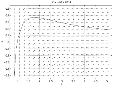
$\begin{equation} \label{e:solntheq} \begin{array}{rcl} \dps \frac{dx}{dt} & = & -\dps \frac{x}{t} + \frac{2}{t^4}\\ x(1) & = & 0. \end{array} \end{equation}$ Compute $H(t)= -\int _1^t\frac {1}{\tau }d\tau = -\ln t +\ln 1 = -\ln t.$ Hence $c(t)=\int _1^t \frac {2}{\tau ^4}e^{\ln \tau }d\tau + 0 =\int _1^t \frac {2}{\tau ^3} d\tau = -\frac {1}{t^2}+1$ which implies that $\begin{equation} \label{e:solnth} x(t)=\left(1-\frac{1}{t^2}\right)\frac{1}{t} \end{equation}$ is the solution. For comparison we show the graph of (??) in Figure ??(left) and the result of a numerical computation of the initial value problem using dfield5 in Figure ??(right).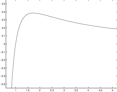

Figure 1: (Left) Graph of solution (??) to equation (??). (Right) The time series for solution to (??) with initial condition $x(1)=0$ using dfield5.

(b) Solve the initial value problem $\begin {array}{rcl} \dps \frac {dx}{dt} & = & 4x + \cos t + e^{2t} \\ x(0) & = & 1. \end {array}$ Here $H(t)=4t$ and

$\begin{eqnarray*} c(t) & = & \int_0^t g(\tau)e^{-4\tau} d\tau +1\\ & = & \int_0^t \left(\cos\tau + e^{2\tau}\right)e^{-4\tau} d\tau +1\\ & = & \frac{1}{17}\left( e^{-4t}(\sin t - 4\cos t)+4\right) + \frac{1}{2}\left(1-e^{-2t}\right) + 1. \end{eqnarray*}$

Thus, the solution is $x(t)=c(t) e^{4t} = \frac {1}{17}(\sin t - 4\cos t+4e^{4t}) - \frac {1}{2}e^{2t} + \frac {3}{2}e^{4t}.$

Exercises

In Exercises ?? – ?? decide whether or not the given differential equation is linear. If it is linear, specify whether the equation is homogeneous or inhomogeneous.

$\dps \frac {dx}{dt} = 0$ .

$\dps \frac {dx}{dt} = x^2\cos t$ .

$\dps \frac {dx}{dt} = x+t^2$ .

$\dps \frac {dx}{dt} = \frac {t}{x}-\frac {1}{t}$ .

$\dps (t^2+1)\frac {dx}{dt} = x+\sin t$ .

$\dps x\frac {dx}{dt} = \cos t$

In Exercises ?? – ?? solve the given initial value problems by variation of parameters.

$\dps \frac {dx}{dt} = t^2 x + t^2, \quad x(1)=1$ .

$\dps \frac {dx}{dt} = x+2t, \quad x(0)=-1$ .

$\dps \frac {dx}{dt} = \frac {t}{t^2+1}x+\sin (t)\sqrt {t^2+1},\quad x(0)=2$ .

$\dps \frac {dx}{dt} = 2x+\frac {1}{t}e^{2t}, \quad x(1)=4$ .

In Exercises ?? – ?? use dfield5 to compute solutions to the given linear differential equations. What is the asymptotic behavior of the solutions as $t$ tends to infinity? Use variation of parameters to explain the behavior.

$\dps \frac {dx}{dt} = -2 x + t$ .

$\dps \frac {dx}{dt} = -2 x + t^2$ .

$\dps \frac {dx}{dt} = -2 x + \sin t$ .