Exact Differential Equations

$\newenvironment {prompt}{}{} \newcommand {\Sec }[2]{\section {#1}} \newcommand {\trademark }[0]{{R\!\!\!\!\!\bigcirc }} \newcommand {\EXER }[0]{\section *{Exercises}} \newcommand {\CEXER }[0]{} \newcommand {\TEXER }[0]{} \newcommand {\R }[0]{\mbox {$\Bbb {R}$}} \newcommand {\C }[0]{\mbox {$\Bbb {C}$}} \newcommand {\Z }[0]{\mbox {$\Bbb {Z}$}} \newcommand {\N }[0]{\mbox {$\Bbb {N}$}} \newcommand {\D }[0]{\mbox {{\bf D}}} \newcommand {\setmin }[0]{\;\mbox {--}\;} \newcommand {\Matlab }[0]{{M\small {AT\-LAB}} } \newcommand {\Matlabp }[0]{{M\small {AT\-LAB}}} \newcommand {\computer }[0]{\Matlab Instructions} \newcommand {\half }[0]{\mbox {$\frac {1}{2}$}} \newcommand {\compose }[0]{\raisebox {.15ex}{\mbox {{\scriptsize $\circ $}}}} \newcommand {\AND }[0]{\quad \mbox {and}\quad } \newcommand {\vect }[2]{\left (\begin {array}{c} #1_1 \\ \vdots \\ #1_{#2}\end {array}\right )} \newcommand {\mattwo }[4]{\left (\begin {array}{rr} #1 & #2\\ #3 &#4\end {array}\right )} \newcommand {\mattwoc }[4]{\left (\begin {array}{cc} #1 & #2\\ #3 &#4\end {array}\right )} \newcommand {\vectwo }[2]{\left (\begin {array}{r} #1 \\ #2\end {array}\right )} \newcommand {\vectwoc }[2]{\left (\begin {array}{c} #1 \\ #2\end {array}\right )} \newcommand {\inv }[0]{^{-1}} \newcommand {\CC }[0]{{\cal C}} \newcommand {\CCone }[0]{\CC ^1} \newcommand {\Span }[0]{{\rm span}} \newcommand {\rank }[0]{{\rm rank}} \newcommand {\trace }[0]{{\rm tr}} \newcommand {\RE }[0]{{\rm Re}} \newcommand {\IM }[0]{{\rm Im}} \newcommand {\nulls }[0]{{\rm null\;space}} \newcommand {\dps }[0]{\displaystyle } \newcommand {\arraystart }[0]{\renewcommand {\arraystretch }{1.8}} \newcommand {\arrayfinish }[0]{\renewcommand {\arraystretch }{1.2}} \newcommand {\Start }[1]{\vspace {0.08in}\noindent {\bf Section~\ref {#1}}} \newcommand {\exer }[1]{\noindent {\bf \ref {#1}}} \newcommand {\ans }[0]{} \newcommand {\matthree }[9]{\left (\begin {array}{rrr} #1 & #2 & #3 \\ #4 & #5 & #6 \\ #7 & #8 & #9\end {array}\right )} \newcommand {\cvectwo }[2]{\left (\begin {array}{c} #1 \\ #2\end {array}\right )} \newcommand {\cmatthree }[9]{\left (\begin {array}{ccc} #1 & #2 & #3 \\ #4 & #5 & #6 \\ #7 & #8 & #9\end {array}\right )} \newcommand {\vecthree }[3]{\left (\begin {array}{r} #1 \\ #2 \\ #3\end {array}\right )} \newcommand {\cvecthree }[3]{\left (\begin {array}{c} #1 \\ #2 \\ #3\end {array}\right )} \newcommand {\cmattwo }[4]{\left (\begin {array}{cc} #1 & #2\\ #3 &#4\end {array}\right )} \newcommand {\thehelp }[0]{\thesection .\arabic {equation}} \newcommand {\matlabEquation }[0]{\let \oldtheequation \theequation \renewcommand {\theequation }{\oldtheequation *}\begin {equation}} \newcommand {\HyperFirstAtBeginDocument }[0]{\AtBeginDocument } \newcommand {\epstopdfsetup }[0]{\setkeys {ETE}} changed the theorem header of amsthm failed\MessageBreak }}} \newcommand {\GetTitleStringSetup }[0]{\setkeys {gettitlestring}} \newcommand {\Sectionformat }[2]{#1}$ $% This file was *autogenerated* from exactDifferentialEquations.sagetex.sage with % sagetex.py version 2015/08/26 v3.0-92d9f7a %a3a9d22459d6eb99bff58ae4b576fbe9% md5sum of corresponding .sage file (minus "goboom","current_tex_line",and pause/unpause lines)$

We illustrate the idea behind exact equations with the following example:

$\begin{equation} \label{eq:exactex1} \frac{dx}{dt} = \frac{x-1}{2x-t}. \end{equation}$ Since the right hand side of (??) is neither of the form $g(x)h(t)$ nor of the form $F\left (\frac {x}{t}\right )$ , it cannot be solved either by separation of variables or by substitution. However, it is possible to determine all solutions of (??), as we now explain.

We may rewrite (??) as

$\begin{equation} \label{eq:exactex1a} (2x-t)\frac{dx}{dt} =(x-1). \end{equation}$

Suppose that $x(t)$ is a solution to (??) and let $y(t)=x(t)^2 - x(t)t + t$ . Then differentiation shows that $\dot {y} = 2x\dot {x} -\dot {x}t-x + 1 = (2x-t)\dot {x} -(x-1) =0,$ with the last equality coming from (??). Thus, if $x(t)$ is a solution, then the function $y(t)=x(t)^2 - x(t)t + t$ is constant. It follows that for each solution $x(t)$ there is a real constant $c$ such that

$\begin{equation} \label{eq:xc} x(t)^2 - x(t)t + t = c. \end{equation}$ Since (??) is quadratic in $x$ , the quadratic formula determines two solutions for each value of $c$ , namely, $\begin{equation} \label{E:twosolns} x_\pm(t) = \frac{t\pm\sqrt{t^2-4t+4c}}{2}. \end{equation}$ When $c=1$ , the radical in (??) is a perfect square and the two solutions to (??) are: $x_+(t) = t-1 \AND x_-(t) = 1,$ as can readily be checked.

Solutions Lie on Level Contours

To derive a geometric interpretation for the identity (??), define the function $F:\R ^2\rightarrow \R$ by $F(t,x) = x^2 - xt + t.$ A level set or contour of $F$ is defined to be the set of points in the $(t,x)$ -plane for which $F(t,x) = c,$ for some real constant $c$ . Thus, (??) can now be restated as follows: solutions $x(t)$ of the differential equation (??) lie on the level sets of $F$ , since $F(t,x(t))=c$ .

Drawing Contours Using MATLAB

We use the MATLAB command contour to illustrate how this information helps us to visualize all the solutions. Type

[t,x] = meshgrid(-1.5:0.1:1.5,-1.5:0.1:1.5);
 
F = x.^2 - x.*t + t;

After these commands the data for the surface defined by the function $F$ in the square $[-1.5,1.5]\times [-1.5,1.5]$ is stored in the MATLAB variable F. The command contour(F) allows us to display the level sets of $F$ . To have the correct scales on the axes, type

contour(t,x,F)

Now the contour lines — the level sets corresponding to different levels $c$ — are displayed. Moreover, we want to know to which levels the curves in that picture belong. Suppose that we are interested in the level sets corresponding to $c\in \{ -2,-1,0,1,2,3,4,5\}$ . Then we obtain this information by typing

cs = contour(t,x,F,[-2,-1,0,1,2,3,4,5]);
 
clabel(cs)
 
xlabel(’t’)
 
ylabel(’x’)

The command clabel allows us to label the different contour lines by their actual level. The desired information is displayed in Figure ??.

Figure 1: Contour lines of $F(t,x)=x^2-xt+t$ for $(t,x)\in [-1.5,1.5]\times [-1.5,1.5]$ .

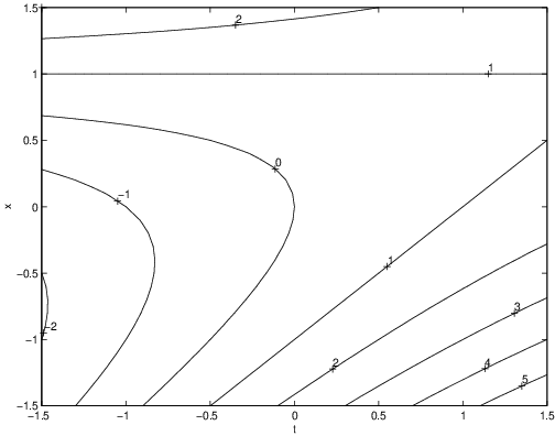
Note that the straight line solutions $x(t)=1$ and $x(t)=t-1$ correspond to the level set for $c=1$ , as expected. We can also see from Figure ?? that the contour lines for the levels $c=0,-1,-2$ have a turning point, that is, they cannot be parameterized entirely by $t$ .

Setting $c=0$ in (??) we find the expressions $x_+(t) = \frac {1}{2}\left (t+\sqrt {t(t-4)}\right ) \AND x_-(t) = \frac {1}{2}\left (t-\sqrt {t(t-4)}\right ).$ These functions are not real-valued for $t\in (0,4)$ . In particular, they cannot correspond to solutions of (??) for these values of $t$ . This provides an explanation for the existence of the turning point at $(t,x)=(0,0)$ and why the solutions $x_+(t)$ and $x_-(t)$ “collide” at this point.

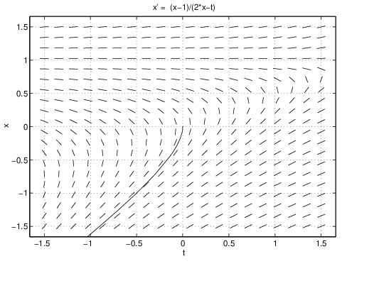
Finally, we use dfield5 to confirm our theoretical discussion. We set the values in the display window as in Figure ?? and start the computation in $(t_0,x_0)=(-0.5,x_-(-0.5))=(-0.5,-1)$ using the Keyboard input. The result — which is in good agreement with the contour plot — is shown in Figure ??. Observe that dfield5 will not stop the computation of the forward orbit on its own and one has to use the Stop button to stop the numerical solution. The reason is that the program encounters numerical difficulties approaching the turning point $(0,0)$ , since the right hand side of the differential equation is not defined at $(0,0)$ .

Figure 2: The solution of (??) for the initial value $(t_0,x_0)=(-0.5,-1)$ computed by dfield5.

The General Definition of Exact Differential Equations

After this motivating example, we consider the general situation. Suppose that we have an ordinary differential equation of the form

$\begin{equation} \label{eq:exact} \frac{dx}{dt} = \frac{G(t,x)}{H(t,x)}, \end{equation}$ where $G$ and $H$ are real-valued continuous functions. In (??), $G(t,x)=x-1$ and $H(t,x) = 2x-t$ . The differential equation (??) is exact if there is a function $F(t,x)$ such that $\begin{equation} \label{e:FGH} \frac{\partial F}{\partial t} = -G \AND \frac{\partial F}{\partial x} = H. \end{equation}$ Indeed, the differential equation (??) is exact — just set $F(t,x) = x^2 - xt + t$ .

Supposing that the differential equation (??) is exact, proceed as in the example by rewriting (??) as

$\begin{equation} \label{eq:exacta} H(t,x)\frac{dx}{dt} - G(t,x) = 0. \end{equation}$ Let $x(t)$ be a solution to (??) and use the chain rule, (??), and (??) to obtain $\frac {d}{dt} F(t,x(t)) = \frac {\partial F}{\partial x}\frac {dx}{dt} + \frac {\partial F}{\partial t} = H\frac {dx}{dt}-G = 0.$ Hence, solutions of (??) must lie on a level set of $F$ defined by $F(t,x) = c$ . We have proved:

Assume that the differential equation (??) is exact. Then, for any solution $x(t)$ of (??) with $x(t_0)=x_0$ , there is a constant $c$ such that for all $t$ close to $t_0$ , $F(t,x(t)) = c$ .

On the Existence of $F$

In order to solve exact differential equations, we must answer two questions:

When does a function $F$ exist that satisfies the conditions in (??)?
If the function $F$ exists, then how can we compute it?

The following proposition, based on the equality of mixed partial derivatives, gives a necessary condition for having a positive answer to the first question.

Let $G,H:\R ^2\to \R$ be differentiable functions such that $\partial G/\partial x$ and $\partial H/\partial t$ are continuous. Suppose that the corresponding differential equation (??) is exact. Then $\begin{equation} \label{eq:Gy=Hs} -\frac{\partial G}{\partial x} (t,x) = \frac{\partial H}{\partial t} (t,x). \end{equation}$

Proof: Using (??) we compute $\frac {\partial ^2 F}{\partial x\partial t} = -\frac {\partial G}{\partial x} (t,x) \AND \frac {\partial ^2 F}{\partial t\partial x} = \frac {\partial H}{\partial t} (t,x).$ Since $\partial G/\partial x$ and $\partial H/\partial t$ are continuous, equality of mixed partial derivatives holds, and $-\frac {\partial G}{\partial x} = \frac {\partial ^2 F}{\partial x\partial t} = \frac {\partial ^2 F}{\partial t\partial x} = \frac {\partial H}{\partial t},$ as desired. $\blacksquare$

It can be shown that criterion (??) is also sufficient for the exactness of the corresponding differential equation, if this criterion is satisfied in a region in the $(t,x)$ -plane having no holes. The proof of this result can be found in any text on multidimensional calculus.

Two Examples

We use two examples to illustrate the test for exactness of the underlying differential equation given by (??).

(a) Consider (??), that is, suppose $G(t,x)=x-1$ and $H(t,x)=2x-t$ . Then $-\frac {\partial G}{\partial x} = -1 = \frac {\partial H}{\partial t},$ and according to Remark ?? a function $F$ with the desired properties may be found.

(b) Suppose that $G(t,x) = 1$ and $H(t,x) = t$ . Then $-\frac {\partial G}{\partial x} (t,x) = 0\not = 1 = \frac {\partial H}{\partial t} (t,x),$ and by Proposition ?? a function $F$ satisfying (??) cannot exist.

On the Computation of $F$

Next, consider the second question, namely, how can $F$ be computed when it exists. By (??) we have $\frac {\partial F}{\partial t}(t,x) = -G(t,x).$ Therefore, there is a differentiable function $g:\R \to \R$ such that

$\begin{equation} \label{eq:defGamma} F(t,x) = -\Gamma(t,x) + g(x), \end{equation}$ where $\Gamma (t,x)=\int G(\tau ,x) d\tau$ is an indefinite integral of $G$ with respect to the variable $t$ . Condition (??) also implies that $H(t,x) = \frac {\partial F}{\partial x}(t,x) = -\frac {\partial }{\partial x}\Gamma (t,x) + g'(x),$ that is $\begin{equation} \label{eq:defg} g'(x) = \frac{\partial}{\partial x}\Gamma(t,x) + H(t,x). \end{equation}$ Equations (??) and (??) can now be used to compute the function $F$ as long as the corresponding integrations can be performed.

Equivalently, we can first integrate the condition $F_x=H$ to obtain

$\begin{equation} \label{eq:excond} F(t,x) = \Omega(t,x) + h(t), \end{equation}$ where $\Omega (t,x)=\int H(t,x)dx$ is an indefinite integral of $H$ with respect to $x$ . Then (??) leads to $h'(t) = -\frac {\partial }{\partial t}\Omega (t,x) - G(t,x).$ In practice, we prefer one way to the other depending on which integrations are easier to perform.

Two Examples

(a) Reconsider (??), that is, suppose $G(t,x)=x-1$ and $H(t,x)=2x-t$ . We can choose $\Gamma (t,x)=\int G(\tau ,y)d\tau = tx-t,$ and (??) becomes $g'(x) = t + H(t,x) = 2x.$ We can then choose $g(x)=x^2$ and, by (??), obtain $F(t,x) = -\Gamma (t,x) + g(x) = -tx + t + x^2.$

(b) Next, consider the differential equation

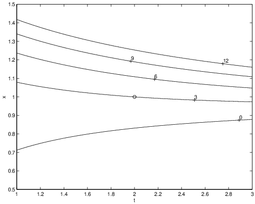
$\begin{equation} \label{eq:exacex2} \frac{dx}{dt} = \frac{2t(1-x^2)-x^6}{x(2t^2+3x+6tx^4)}. \end{equation}$ In our notation $G(t,x) = 2t(1-x^2)-x^6 \AND H(t,x) = x(2t^2+3x+6tx^4).$ Therefore, $-\frac {\partial G}{\partial x} = 4tx + 6x^5 = \frac {\partial H}{\partial t}.$ Hence the equation is exact (see Proposition ?? and Remark ??).

It is easier to compute $\Gamma (t,x)=\int G(\tau ,x) d\tau$ than $\Omega (t,x)=\int H(s,x)dx$ . We choose $\Gamma (t,x) = t^2(1-x^2) - tx^6,$ and (??) becomes $g'(x) = -(2t^2 x + 6tx^5) + x(2t^2+3x+6tx^4) = 3x^2.$ Now we use (??) to obtain $F(t,x) = t^2(x^2-1) + tx^6 + x^3.$ Solutions of the differential equation (??) lie on level sets of $F$ . In particular, the solution $x(t)$ determined by the initial condition $x(2)=1$ satisfies $F(t,x)=t^2(x^2-1) + tx^6 + x^3 = 3,$ since $F(2,1)=3$ . To see the qualitative behavior of the solutions we use the following sequence of MATLAB commands

[t,x] = meshgrid(1:0.02:3,0.5:0.01:1.5);
 
F  = t.^2.*(x.^2-1) + t.*x.^6 + x.^3;
 
cs = contour(t,x,F,[0,3,6,9,12]);
 
clabel(cs)
 
hold on
 
plot(2,1,’o’)
 
xlabel(’t’)
 
ylabel(’x’)

The result is shown in Figure ??.

Figure 3: Solutions of the differential equation (??) corresponding to the levels $c=0,3,6,9,12$ in the rectangle $[1,3]\times [0.5,1.5]$ .

Exercises

In Exercises ?? – ?? determine whether or not the given differential equations is exact.

$\dps \frac {dx}{dt} = \frac {\cos x}{t\sin x}$ .

$\dps \frac {dx}{dt} = \frac {\cos t}{x\sin t}$ .

Verify that the differential equation $\dps \frac {dx}{dt} = \dps \frac {2t-x}{t+1}$ is exact and find a solution with initial value $x(0) = 3$ .

Verify that the differential equation $\frac {dx}{dt} = \frac {x}{x-t}$ is exact and find a solution with initial value $x(2)=3$ . Compare your answer with Exercise ?? in Section ??.

Show that the differential equation $\begin{equation} \label{Ex:nexact} \frac{dx}{dt} = -\frac{1+3tx}{t^2} \end{equation}$ is not exact. Now multiply both the numerator and denominator of the right side of (??) by $t$ and show that this ‘new’ differential equation $\frac {dx}{dt} = -\frac {t+3t^2x}{t^3}$ is exact. Now find all solutions to (??).

Show that the differential equation $\begin{equation} \label{Ex:nexact2} \frac{dx}{dt} = -\frac{3x}{2t} \end{equation}$ is not exact. Now multiply both the numerator and denominator of the right side of (??) by $t^2x$ and show that this ‘new’ differential equation $\frac {dx}{dt} = -\frac {3t^2x^2}{2t^3x}$ is exact. Now find all solutions to (??).

Let $G,H:\R ^2\to \R$ be continuous functions and suppose that the differential equation $\begin{equation} \label{eq:if1} \frac{dx}{dt} = \frac{G(t,x)}{H(t,x)} \end{equation}$ is not exact. An integrating factor for (??) is a function $\rho :\R ^2\rightarrow \R$ such that the differential equation $\frac {dx}{dt} = \frac {\rho (t,x) G(t,x)}{\rho (t,x)H(t,x)}$ is exact. Suppose that there exists an integrating factor $\rho (t)$ for (??) that is a function of $t$ alone. Show that $\rho$ satisfies $\frac {d\rho }{dt} = -\frac {\rho }{H} \left ( \frac {\partial G}{\partial x}+\frac {\partial H}{\partial t}\right ).$

Use the result of Exercise ?? to find an integrating factor for the differential equation $\frac {dx}{dt} = -\frac {8x+5t}{4t},$ and then determine all solutions of this differential equation.

Consider the differential equation $\frac {dx}{dt} = -\frac {2tx+\cos x}{t(t-\sin x)}.$ Show that this differential equation is exact. Then use the command contour in MATLAB to find solutions. For the display, use the rectangle $[-2,2]\times [-2,2]$ in the $(t,x)$ -plane and show contour lines for the different levels $c=-4,-3,-2,-1,0,1,2,3,4$ . Mark the solution which satisfies the initial condition $x(1)=0$ by a circle. Hint: Use the same procedure that was used to create Figure ??.

Solutions Lie on Level Contours

Drawing Contours Using MATLAB

The General Definition of Exact Differential Equations

On the Existence of <![CDATA[ F ]]>

Two Examples

On the Computation of <![CDATA[ F ]]>

Two Examples

Exercises

On the Existence of $F$

On the Computation of $F$