Previously, we have used dfield5, pline, and pplane5 to compute solutions to one and two dimensional ordinary differential equations numerically. We now wish to compute solutions to higher dimensional systems of ordinary differential equations and to do this we will use the MATLAB command ode45. MATLAB provides the command ode45, among others, for solving initial value problems, and we illustrate how this command works on several examples. In this section we illustrate the command on a simple one dimensional example and in the next section we will compute solutions to three and four dimensional systems.
A Simple One Dimensional Example
Suppose that we want to compute numerically the solution of the initial value problem
on the time interval . Then the data of this problem are- the numbers and , and
- the function .
We know how to assign specific values for and in MATLAB; we will call these variables t0, x0 and te. Before proceeding, we need to understand how to make a function available for computations in MATLAB.
The Construction of m-files in MATLAB
Functions that are used by MATLAB are defined via m-files. We now show how to construct m-files with two examples.
Suppose that we want the function , defined by
for . In this case, , , and . After typing the command[t,x] = ode45(’f14_3_4’,[1 3],2);the approximate solution is stored in the vectors t and x. The components of the vector t are the values of for which the solution has been computed, and the components of the vector x are the values of the solution at the values t. Indeed, typing t and x we see that both vectors have length . The length of the vectors t and x is chosen by ode45 so as to guarantee a certain accuracy in the solution. We discuss this issue in greater detail below.
We can visualize the solution by plotting its time series:
plot(t,x)

xlabel(’t’)

ylabel(’x’)
The result is shown in Figure ??.
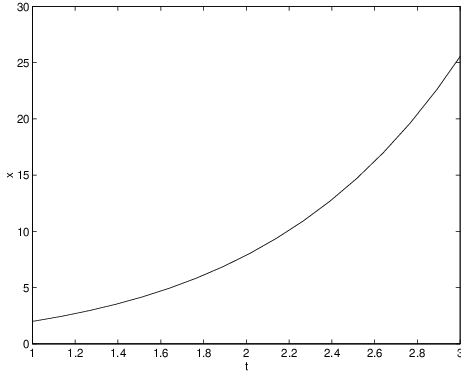
In fact, the initial value problem (??) has a simple closed form solution which can be verified directly by differentiation. The existence of this closed form solution allows us to check the accuracy of the numerical calculations made by ode45. Indeed, graphically we cannot distinguish the result obtained using ode45 from the exact solution. To verify this point, type
x_exact = 4*exp(t-1)-t-1;and observe that the graph of the exact solution, which is in red, exactly covers the plot of the numerically computed solution.
hold on
plot(t,x_exact,’r’)
Accuracy of ode45
We now discuss the error made by ode45 in more detail. Using ode45 we obtained an approximation of the solution of the initial value problem (??) at the times for . The exact solution at these points is and the ode45 approximation to the solution is . The routine ode45 automatically computes the solution subject to satisfying two constraints: absolute error and relative error.
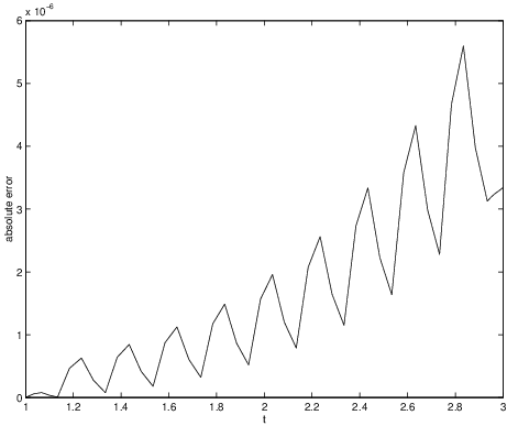
The absolute error is just the absolute value of the difference between the numerically computed solution and the exact solution, that is, We can visualize the absolute error by plotting versus , as follows:
err_abs = abs(x-x_exact);The MATLAB command abs(v) generates a vector containing the absolute values of the components of the vector v. The result is presented in Figure ??. Note that even though the absolute error oscillates, it is always less than , which is why we could not distinguish the graph of the exact solution from the graph of the numerically computed solution given in Figure ??.
plot(t,err_abs)
xlabel(’t’)
ylabel(’absolute error’)
Having an absolute error of in a numerically computed solution might seem quite good — unless we happened to be computing a solution whose size is . Then the numerical error would be ten times the size of the solution itself, which is a huge error. For this reason, numerical analysts like to use another measure for success.
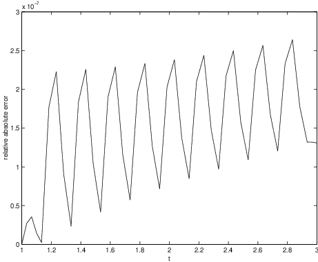
The relative error between the approximation and the exact solution is the absolute error normalized by the size of the exact solution, that is The numbers must be uniformly small in order to guarantee a good numerical approximation to the actual solution. Using the fact that we have a formula for the exact solution, we can compute the numbers and plot them in MATLAB by typing
err_rel = abs(x-x_exact)./abs(x_exact);The result is shown in Figure ??. We see that the relative error oscillates, but is always smaller than .
plot(t,err_rel)
xlabel(’t’)
ylabel(’relative error’)
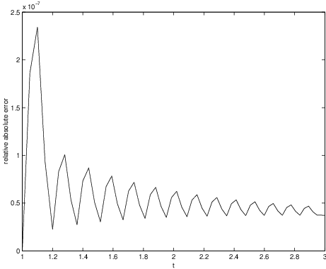
Default error bounds are preset in the command ode45. Unless otherwise instructed ode45 attempts to find a numerical approximation whose absolute error is everywhere less than and whose relative error is everywhere less than . (There is a interesting mathematical question concerning how these bounds are actually satisfied, since ode45 does not, in fact, know the exact solution.) We can use ode45 to compute an approximation of the solution with an even smaller error. To set this smaller error, we add an argument to the call of ode45 by typing
options = odeset(’RelTol’,1e-8);These instructions compute an approximation for which the relative error is smaller than . (Type odeset in MATLAB in order to see a complete list of options. Type options to see a list of the currently specified options.) Hence, when we perform this calculation, we expect to obtain an even better result than before. Indeed, proceeding as above, we obtain the relative error shown in Figure ??. In an attempt to guarantee the reduced error, ode45 generates 61 time steps during the computation.
[t,x]=ode45(’f14_3_4’,[1 3],2,options);
Exercises
For each function specified in Exercises ?? – ??, write an m-file that makes that function available in MATLAB.