A Description of Numerical Methods

$\newenvironment {prompt}{}{} \newcommand {\Sec }[2]{\section {#1}} \newcommand {\trademark }[0]{{R\!\!\!\!\!\bigcirc }} \newcommand {\EXER }[0]{\section *{Exercises}} \newcommand {\CEXER }[0]{} \newcommand {\TEXER }[0]{} \newcommand {\R }[0]{\mbox {$\Bbb {R}$}} \newcommand {\C }[0]{\mbox {$\Bbb {C}$}} \newcommand {\Z }[0]{\mbox {$\Bbb {Z}$}} \newcommand {\N }[0]{\mbox {$\Bbb {N}$}} \newcommand {\D }[0]{\mbox {{\bf D}}} \newcommand {\setmin }[0]{\;\mbox {--}\;} \newcommand {\Matlab }[0]{{M\small {AT\-LAB}} } \newcommand {\Matlabp }[0]{{M\small {AT\-LAB}}} \newcommand {\computer }[0]{\Matlab Instructions} \newcommand {\half }[0]{\mbox {$\frac {1}{2}$}} \newcommand {\compose }[0]{\raisebox {.15ex}{\mbox {{\scriptsize $\circ $}}}} \newcommand {\AND }[0]{\quad \mbox {and}\quad } \newcommand {\vect }[2]{\left (\begin {array}{c} #1_1 \\ \vdots \\ #1_{#2}\end {array}\right )} \newcommand {\mattwo }[4]{\left (\begin {array}{rr} #1 & #2\\ #3 &#4\end {array}\right )} \newcommand {\mattwoc }[4]{\left (\begin {array}{cc} #1 & #2\\ #3 &#4\end {array}\right )} \newcommand {\vectwo }[2]{\left (\begin {array}{r} #1 \\ #2\end {array}\right )} \newcommand {\vectwoc }[2]{\left (\begin {array}{c} #1 \\ #2\end {array}\right )} \newcommand {\inv }[0]{^{-1}} \newcommand {\CC }[0]{{\cal C}} \newcommand {\CCone }[0]{\CC ^1} \newcommand {\Span }[0]{{\rm span}} \newcommand {\rank }[0]{{\rm rank}} \newcommand {\trace }[0]{{\rm tr}} \newcommand {\RE }[0]{{\rm Re}} \newcommand {\IM }[0]{{\rm Im}} \newcommand {\nulls }[0]{{\rm null\;space}} \newcommand {\dps }[0]{\displaystyle } \newcommand {\arraystart }[0]{\renewcommand {\arraystretch }{1.8}} \newcommand {\arrayfinish }[0]{\renewcommand {\arraystretch }{1.2}} \newcommand {\Start }[1]{\vspace {0.08in}\noindent {\bf Section~\ref {#1}}} \newcommand {\exer }[1]{\noindent {\bf \ref {#1}}} \newcommand {\ans }[0]{} \newcommand {\matthree }[9]{\left (\begin {array}{rrr} #1 & #2 & #3 \\ #4 & #5 & #6 \\ #7 & #8 & #9\end {array}\right )} \newcommand {\cvectwo }[2]{\left (\begin {array}{c} #1 \\ #2\end {array}\right )} \newcommand {\cmatthree }[9]{\left (\begin {array}{ccc} #1 & #2 & #3 \\ #4 & #5 & #6 \\ #7 & #8 & #9\end {array}\right )} \newcommand {\vecthree }[3]{\left (\begin {array}{r} #1 \\ #2 \\ #3\end {array}\right )} \newcommand {\cvecthree }[3]{\left (\begin {array}{c} #1 \\ #2 \\ #3\end {array}\right )} \newcommand {\cmattwo }[4]{\left (\begin {array}{cc} #1 & #2\\ #3 &#4\end {array}\right )} \newcommand {\thehelp }[0]{\thesection .\arabic {equation}} \newcommand {\matlabEquation }[0]{\let \oldtheequation \theequation \renewcommand {\theequation }{\oldtheequation *}\begin {equation}} \newcommand {\HyperFirstAtBeginDocument }[0]{\AtBeginDocument } \newcommand {\epstopdfsetup }[0]{\setkeys {ETE}} changed the theorem header of amsthm failed\MessageBreak }}} \newcommand {\GetTitleStringSetup }[0]{\setkeys {gettitlestring}} \newcommand {\Sectionformat }[2]{#1} \newcommand {\arraystretch }[0]{1.8} \newcommand {\arraystretch }[0]{1.2} \newcommand {\arraystretch }[0]{1.8} \newcommand {\arraystretch }[0]{1.2} \newcommand {\arraystretch }[0]{1.8} \newcommand {\arraystretch }[0]{1.2} \newcommand {\arraystretch }[0]{1.8} \newcommand {\arraystretch }[0]{1.2} \newcommand {\arraystretch }[0]{1.8} \newcommand {\arraystretch }[0]{1.2} \newcommand {\arraystretch }[0]{1.8} \newcommand {\arraystretch }[0]{1.2}$ $% This file was *autogenerated* from aDescriptionOfNumericalMethods.sagetex.sage with % sagetex.py version 2015/08/26 v3.0-92d9f7a %fe04e0440213071529d5ca9d6a97a577% md5sum of corresponding .sage file (minus "goboom","current_tex_line",and pause/unpause lines)$

By definition, derivatives are limits of Newtonian quotients and approximating this limit provides one of the basic ideas in the construction of numerical methods. More precisely, let $x$ be the solution of the initial value problem $\dot x = f(t,x)$ , $x(t_0)=x_0$ . The derivative of $x$ at time $t$ is the limit $\frac {dx}{dt}(t) = \lim _{h\to 0} \frac {x(t+h) - x(t)}{h}.$ Hence we expect

$\begin{equation} \label{eq:eul1} x(t+h) \approx x(t) + h \frac{dx}{dt}(t) = x(t) + h f(t,x(t)) \end{equation}$ to be a good approximation of $x$ at time $t+h$ for small $h$ . Indeed, by Taylor’s formula $\begin{equation} \label{eq:tfeul} \begin{array}{rcl} \dps x(t+h)&=& \dps x(t)+h\frac{dx}{dt}(t)+\frac{h^2}{2}\frac{d^2x}{dt^2}(t+\theta h)\\ &=& \dps x(t)+hf(t,x(t))+\frac{h^2}{2}\frac{d^2x}{dt^2}(t+\theta h), \end{array} \end{equation}$ with an appropriate $0<\theta <1$ . Thus, the error made in the approximation in (??) is the size $h^2$ as long as the second derivative of $x(t)$ is bounded. Consequently, if we know the value of the solution $x$ at time $t$ , then we can use the right hand side $f$ in the differential equation to compute an approximation of the solution $x$ at time $t+h$ .

Euler’s Method

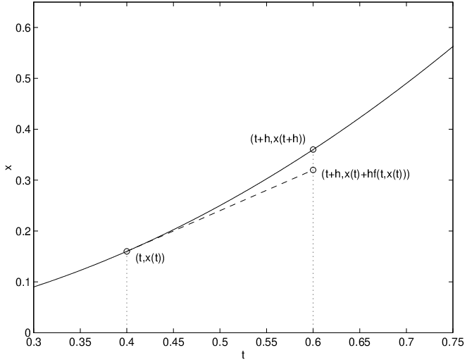
Since $f(t,x(t))$ is the derivative of $x$ at time $t$ , there is a simple geometric interpretation of (??) (see Figure ??). Recall that the tangent line to the graph of the function $x(t)$ at the point $(t,x(t))$ is the line going through the point $(t,x(t))$ whose slope is $\dot {x}(t)=f(t,x(t))$ . The approximation of $x$ at time $t+h$ is just the one given by the value of that tangent line at $t+h$ . The numerical method that is based on (??) is called Euler’s method. It seems evident that smaller values of $h$ should lead to a more accurate approximation of the solution $x$ on the interval $[t,t+h]$ . On the other hand, note that simultaneously the length of the interval $[t,t+h]$ is shrinking and that more approximations are needed to approximate a solution on a fixed time interval.

Figure 1: Illustration of one step in Euler’s method for $h=0.2$ .

Concretely, Euler’s method produces a sequence of approximations to a solution of an initial value problem. To understand this point, begin the numerical integration at the exact initial value $(t_0,x_0)$ . Choose a step size $h>0$ . Use (??) to obtain after one integration step the approximation $x(t_1)\approx x_1$ where $t_1 = t_0+h \AND x_1 = x_0 + h f(t_0, x_0).$ Continuing this process, construct a sequence

$\begin{equation} \label{eq:eulmethod} t_{k+1} = t_k+h \AND x_{k+1} = x_k + h f(t_k, x_k) \end{equation}$ for $k=0,1,\ldots ,K-1$ where $K$ is the total number of steps that are performed in the numerical approximation.

An Example of Euler’s Method

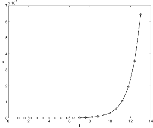
We illustrate how Euler’s method works for the example

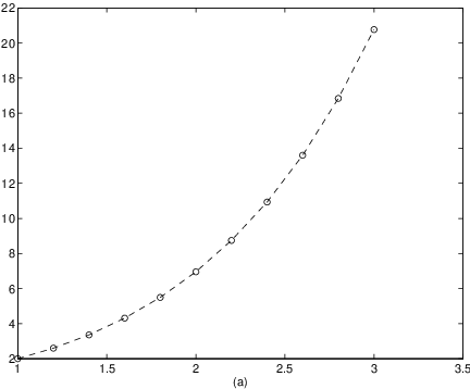
$\begin{equation} \label{eq:eulexivp} \begin{array}{rcl} \dps\frac{dx}{dt} & = & x+t\\ x(1) & = & 2, \end{array} \end{equation}$ by using MATLAB to compute an approximation to $x(3)$ . Suppose that we set the step size to $h = 0.2$ . Then the number of steps needed to reach $t=3$ is $K=10$ . The code for computing the sequence in (??) is:

h    = 0.2;
 
t(1) = 1;
 
x(1) = 2;
 
K    = 10;
 
for k = 1:K
 
   t(k+1) = t(k)+h;
 
   x(k+1) = x(k)+h*(x(k)+t(k));
 
end
 
plot(t,x,’o’)
 
hold on
 
plot(t,x,’--’)
 
xlabel(’(a)’)

The result is shown in Figure ??(a). Note that the ’o’ in the MATLAB command plot(t,x,’o’) puts o’s at the 11 numerically computed points and the ’- -’ in the command plot(t,x,’--’) interpolates dashed lines between successive o’s. Moreover, the statements within the for loop — that is the lines from for k = 1:K up to the end — reproduce the iteration procedure given in (??). (In MATLAB the index of a vector is not allowed to be zero. Therefore, the for loop is programmed to run from $k=1,\ldots ,K$ rather than from $k=0,\ldots ,K-1$ .)

Comparison of Numerical Solutions with Exact Solutions

We now compare the numerical approximation with the exact solution of (??), that is given by $x(t) = 4e^{t-1}-t-1.$ This comparison is made in Figure ??(b). The second curve in the figure is obtained using the additional commands

s = 1 : 0.01 : 3;
 
y = 4*exp(s-1)-s-1;
 
plot(s,y)
 
xlabel(’(b)’)

Note that in that figure the scale on the vertical axis is different from the one in Figure ??(a).

Figure 2: Approximation of the solution of (??) by Euler’s method. (a) Circles mark the computed points; dashed lines are linear interpolations between the o’s. (b) A comparison is made to the exact solution pictured as a solid line.

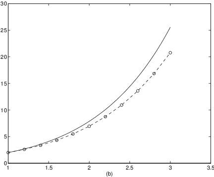
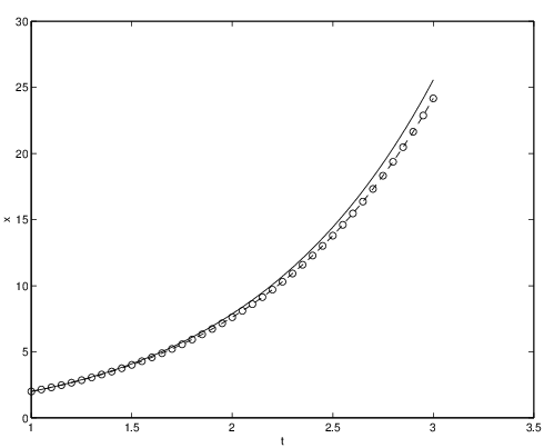
In this example we see that after just $10$ steps the numerical solution of the initial value problem by Euler’s method has led to a significant error (see Figure ?? (b)). There are two ways to proceed. Either we can use a smaller step size in Euler’s method in an attempt to improve accuracy or we can develop numerical methods that give more precise results for the same step size. For an illustration of the first approach we show in Figure ?? an approximation with Euler’s method using a step size $h=0.05$ . It can be seen that the error is now indeed much smaller but that also quite a few iterations of Euler’s method are needed to produce this result. Therefore the latter approach has generally proved preferable and one idea for improving accuracy is to replace $f(t_k,x_k)$ in the right hand side of (??) by another expression in ways that we now explain.

Figure 3: Approximation of the solution of (??) by Euler’s method with step size $h=0.05$ . (Marks and lines as in Figure ??.)

Implicit Methods

In Euler’s method, the approximation $x_{k+1}$ is computed using the tangent line to the graph of the solution at the point $(t_k,x_k)$ . Another idea is to approximate the graph of $x(t)$ by the line passing through the point $(t_k,x_k)$ whose slope is $f(t_{k+1},x_{k+1})$ . This idea leads to the numerical approximation $t_{k+1} = t_k+h \AND x_{k+1} = x_k + h f(t_{k+1}, x_{k+1})$ which is known as the implicit Euler method. One difficulty with this method is that we do not yet know what the value of $x_{k+1}$ is. However, it is implicitly defined in the sense that we can think of the iteration step

$\begin{equation} \label{eq:impleulit} x_{k+1} = x_k + h f(t_{k+1}, x_{k+1}) \end{equation}$ as an equation in the unknown $x_{k+1}$ and use this nonlinear equation to solve for $x_{k+1}$ . We remark that there are ODEs (e.g. so-called stiff equations) for which implicit schemes typically produce more reliable results. On the other hand, implicit methods require considerable additional numerical effort at each time step in order to solve the equations for $x_{k+1}$ .

An implicit numerical method that is more accurate than implicit Euler is obtained by just averaging the Euler and implicit Euler approximations, to obtain

$\begin{equation} \label{eq:imtrap} t_{k+1} = t_k+h \AND x_{k+1} = x_k + \frac{h}{2} \Big( f(t_k, x_k)+f(t_{k+1}, x_{k+1})\Big). \end{equation}$ This method is called the implicit trapezoidal rule.

The Modified Euler Method

As we discussed, the problem with implicit methods is that they require the solution of a nonlinear equation at each time step. In principle this can also be done numerically, but such solutions require much numerical effort. This problem can partly be overcome by using a clever idea discovered by Runge (1895). We illustrate this idea on the implicit trapezoidal rule. Rather than determining $x_{k+1}$ directly from (??), first estimate $x_{k+1}$ by $y_{k+1}$ using Euler’s (tangent line) method. Then use the estimate $y_{k+1}$ in the implicit trapezoidal rule. In formulas we obtain: $t_{k+1} = t_k+h \AND \left \{\begin {array}{rcl} y_{k+1} & = & x_k + h f(t_k, x_k)\\ x_{k+1} & = & x_k + \frac {h}{2} \Big ( f(t_k, x_k)+f(t_{k+1}, y_{k+1})\Big ), \end {array}\right .$ or, in one line,

$\begin{equation} \label{eq:meulmethod} t_{k+1} = t_k+h \AND x_{k+1} = x_k + \frac{h}{2} \Big( f(t_k, x_k)+f(t_{k+1}, x_k + h f(t_k, x_k))\Big). \end{equation}$ The resulting numerical method is called the modified Euler method.

Let us use MATLAB to solve the initial value problem (??) by the modified Euler method. Using the same data as in the previous example we type

h    = 0.2;
 
t(1) = 1;
 
x(1) = 2;
 
K    = 10;
 
for k = 1:K
 
   t(k+1) = t(k)+h;
 
   y(k)   = x(k)+h*(x(k)+t(k));
 
   x(k+1) = x(k)+(h/2)*(x(k)+t(k)+y(k)+t(k+1));
 
end
 
plot(t,x,’o’)
 
hold on
 
plot(t,x,’--’)
 
s = 1 : 0.01 : 3;
 
y = 4*exp(s-1)-s-1;
 
plot(s,y)
 
xlabel(’(a)’)

to obtain the illustration in Figure ??(a). We see that the approximation can hardly be distinguished from the exact solution. Even if we double the step size to $h=0.4$ and reduce the number of steps to $K=5$ , the approximation is still acceptable. See Figure ??(b).

Figure 4: Approximations of the solution of (??) by the modified Euler method with step sizes: (a) $h=0.2$ ; (b) $h=0.4$ . The exact solution is shown with a solid line.

Fourth Order Runga-Kutta Method

The idea in the construction of the modified Euler method is to obtain a better approximation of the solution by using more information on the underlying differential equation. This is realized in the scheme by taking the arithmetic average of two evaluations of the right hand side $f$ at different points rather than at just one point as in the standard Euler methods.

In the frequently used fourth order Runge-Kutta method four different evaluations of $f$ are taken into account in the computation of the next iterate. The method is given as follows: set

$\begin{eqnarray*} f_1 &=& f(t_k,x_k)\\ f_2 &=& f\left(t_k+\frac{h}{2},x_k+\frac{h}{2}f_1\right)\\ f_3 &=& f\left(t_k+\frac{h}{2},x_k+\frac{h}{2}f_2\right)\\ f_4 &=& f(t_k+h,x_k+hf_3), \end{eqnarray*}$

and define the new approximation by $x_{k+1} = x_k+\frac {h}{6}(f_1+2f_2+2f_3+f_4).$ By this method we can approximate solutions of differential equations in a very precise way. We illustrate this by an application to the initial value problem (??). In Figure ?? we show the approximation obtained with the step size $h=0.6$ for $K=20$ steps. The result is particularly convincing — observe that in contrast to Figures ??–?? the solution is approximated on a significantly larger interval.

Figure 5: Approximation of the solution of (??) obtained by the fourth order Runge-Kutta method. The exact solution is superimposed (solid line).

Systems of Differential Equations

All the methods we have introduced in this section can also be used to find numerically solutions of systems of differential equations. We illustrate this fact for systems of two equations using Euler’s method.

In the scalar case the underlying idea for Euler’s method was to approximate the solution of the differential equation over a short interval by a line that is tangent to the solution curve (see Figure ??). We now use the same approach by applying this idea to each component of the solution.

Suppose that $(x(t),y(t))$ is a solution of the initial value problem

$\begin{equation} \label{eq:numanalsys} \begin{array}{rcl} \dps \frac{dx}{dt} & = & f(t,x,y)\\ \dps \frac{dy}{dt} & = & g(t,x,y), \end{array} \end{equation}$ where $(x(t_0),y(t_0))= (x_0,y_0)$ . As in (??) we obtain for the components $x(t)$ and $y(t)$ by using the differential equation

$\begin{eqnarray*} x(t+h) & \approx & x(t) + h \frac{dx}{dt}(t) = x(t) + h f(t,x(t),y(t))\\ y(t+h) & \approx & y(t) + h \frac{dy}{dt}(t) = y(t) + h g(t,x(t),y(t)). \end{eqnarray*}$

Again $h>0$ is called the step size. We can now proceed as in the case of a scalar differential equation and obtain in analogy to (??)

$\begin{eqnarray*} t_{k+1} = t_k+h \AND \left\{\begin{array}{rcl} x_{k+1} &=& x_k + h f(t_k,x_k,y_k)\\ y_{k+1} &=& y_k + h g(t_k,x_k,y_k) \end{array}\right. \quad (k=0,1,\ldots,K-1). \end{eqnarray*}$

Using vector notation Euler’s method applied to the initial value problem (??) can be written as $\begin{equation} \begin{array}{rcl} \vectwo{x_{k+1}}{y_{k+1}} & = & \vectwo{x_k}{y_k} + h \vectwo{f(t_k,x_k,y_k)}{g(t_k,x_k,y_k)}\\ t_{k+1} & = & t_k + h, \end{array} \end{equation}$ for $k=0,1,\ldots ,K$ .

Similarly, the implicit Euler method takes the form

$\begin{eqnarray*} \vectwo{x_{k+1}}{y_{k+1}} & = & \vectwo{x_k}{y_k} + h \vectwo{f(t_{k+1},x_{k+1},y_{k+1})}{g(t_{k+1},x_{k+1},y_{k+1})}\\ t_{k+1} &=& t_k + h. \end{eqnarray*}$

Let us use MATLAB to compute an approximation of the initial value problem $\begin{equation} \label{eq:numanalex1} \begin{array}{rcl} \dps \frac{dx}{dt} & = & y-3t\\ \dps \frac{dy}{dt} & = & y+x^2, \end{array} \end{equation}$ where $(x(1),y(1))= (0,2)$ . We specify the step size $h=0.05$ and find an approximation on the interval $[1,3]$ by typing

h    = 0.05;
 
t(1) = 1;
 
x(1) = 0;
 
y(1) = 2;
 
K    = 40;
 
for k = 1:K
 
   t(k+1) = t(k)+h;
 
   x(k+1) = x(k)+h*(y(k)-3*t(k));
 
   y(k+1) = y(k)+h*(y(k)+x(k)^2);
 
end
 
plot(x,y,’o’)
 
hold on
 
plot(x,y,’--’)
 
xlabel(’x’)
 
ylabel(’y’)

The result is shown in Figure ??.

Figure 6: Approximation of the solution of (??) by Euler’s method with step size $h=0.05$ . The single points of the approximation are marked by circles.

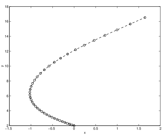
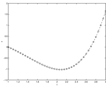
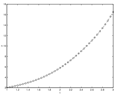
Observe that the solution $(x(t),y(t))$ is graphed in the $xy$ -plane. In particular, the variable $t$ does not appear in the figure and this is the reason why the single steps in the approximation do not seem to be equally spaced. However, in Figure ?? we show graphs of the approximations of the time series $x$ vs. $t$ and $y$ vs. $t$ . Here it can be seen that the step size is indeed constant.

Figure 7: Approximation of the $x$ - and $y$ -components of the solution of (??) by Euler’s method with step size $h=0.05$ .

There are several ways to improve the accuracy of numerical schemes approximating solutions of initial value problems. One very successful method is to adapt the step size $h$ in each step of the numerical approximation. We illustrate this strategy in Appendix ??.

General Runga-Kutta Methods

The modified Euler method as well as the fourth order Runge-Kutta method are specific examples of a general class of numerical schemes for the solution of initial value problems. These schemes are called Runge-Kutta methods. A general explicit Runge-Kutta method is fully described by numbers $b_1,\ldots ,b_s\AND c_1,\ldots ,c_s,$ and $a_{pq}, \quad p=2,\ldots ,s,\quad q=1,\ldots ,p-1.$ With these numbers the $k^{th}$ step in the numerical solution of an initial value problem using a Runge-Kutta method can be described as follows. Given $(t_k,x_k)$ first evaluate $f$ for $s$ times:

$\begin{eqnarray*} f_1 & = & f\left( t_k+c_1 h, x_k \right)\\ f_2 & = & f\left( t_k+c_2 h, x_k +ha_{21} f_1\right)\\ f_3 & = & f\left( t_k+c_3 h, x_k +h(a_{31} f_1 + a_{32} f_2)\right)\\ & \vdots &\\ f_s & = & f\left( t_k+c_s h, x_k +h\sum_{j=1}^{s-1}a_{ij} f_j\right). \end{eqnarray*}$

Second, obtain the next approximation by a weighted average of $f_1,\ldots ,f_s$ : $t_{k+1} = t_k+h \AND x_{k+1} = x_k + h\sum _{i=1}^s b_i f_i.$ We now show that — except for the implicit schemes — all the methods that we have discussed are Runge-Kutta methods.

Euler’s method: set $s=1,\quad b_1=1,\quad c_1=0$ and there are no $a_{pq}$ ’s.
The modified Euler method: set $s=2,\quad b_1=b_2=1/2,\quad c_1=0,\quad c_2=1,\quad a_{21}=1.$ Indeed, using these data
$\begin{eqnarray*} f_1 &=& f(t_k,x_k)\\ f_2 &=& f(t_{k+1},x_k+hf_1)=f(t_{k+1},x_k+hf(t_k,x_k)), \end{eqnarray*}$
and
$\begin{eqnarray*} x_{k+1} &=& x_k + h \left(\frac{1}{2}f_1 + \frac{1}{2}f_2\right)\\ &=& x_k + \frac{h}{2} \Big( f(t_k, x_k)+f(t_{k+1}, x_k + h f(t_k, x_k))\Big). \end{eqnarray*}$
Hence we have obtained (??).
Fourth order Runge-Kutta method: set $s=4,\quad b_1=b_4=1/6,\quad b_2=b_3=2/6,\quad c_1=0,\quad c_2=c_3=1/2,\quad c_4=1,$ and $a_{21}=1/2,\quad a_{31}=0,\quad a_{32}=1/2,\quad a_{41}=0,\quad a_{42}=0,\quad a_{43}=1.$

Exercises

Consider the initial value problem $\begin {array}{rcl} \dps \frac {dx}{dt}(t) & = & -2 \\ x(t_0) & = & 0. \end {array}$ Show that in this case an application of Euler’s method leads to exact results for all step sizes $h$ , that is $x_k=x(t_k)$ for all $k$ .

Write down the implicit trapezoidal rule for the initial value problem (??).

In Exercises ?? – ?? decide whether or not the following numerical schemes are Runge-Kutta methods.

$x_{k+1} = x_k + hf(t_k+\frac {h}{2},x_k+\frac {h}{2}f(t_k,x_k))$ .

$x_{k+1} = x_k + hf(t_k,x_k+t_k)$ .

$x_{k+1} = x_k + \frac {h}{4}(f(t_k,x_k)+3f(t_k+\frac {2h}{3},x_k+\frac {2h}{3}f(t_k,x_k))$ .

Consider the initial value problem $\begin {array}{rcl} \dps \frac {dx}{dt}(t) & = & 1 \\ x(t_0) & = & 0. \end {array}$

Suppose that a Runge-Kutta method leads to exact results for all step sizes $h$ , that is $x_k=x(t_k)$ . What does this imply for the numbers $b_1,\ldots ,b_s$ ?
Verify that the relation on the numbers $b_1,\ldots ,b_s$ derived in part (a) is satisfied for Euler’s method, for the modified Euler method and for the fourth order Runge-Kutta method.

Use formula (??) to show that the first step in the numerical approximations shown in Figures ??(b) and ?? have to lie below the graph of the exact solution $x(t)$ .

Use MATLAB to reproduce the result displayed in Figure ??.

In Exercises ?? – ?? solve the given initial value problem by the explicit and the modified Euler method. Approximate the solution on the given interval and use the prescribed step size $h$ .

$\dot x = 1$ , $x(2)=3$ , step size $h=0.1$ , interval $[2,4]$ .

$\dot x = x^2$ , $x(1)=0.5$ , step size $h=0.2$ , interval $[1,3]$ .

$\dot x = tx$ , $x(1)=-1$ , step size $h=0.05$ , interval $[1,3]$ .

Use MATLAB to solve the initial value problem $\frac {dx}{dt} = x,\quad x(0)=1$ (a) by the implicit Euler method, and (b) by the implicit trapezoidal rule on the interval $[0,2]$ . In each case use the step size $h=0.1$ . Hint: Before working with MATLAB, use this specific differential equation to solve explicitly for $x_{k+1}$ in (??) and (??).

Program the fourth order Runge-Kutta method in MATLAB to verify the numerical computation in Figure ??. Compare the results to those obtained by ode45.

Use MATLAB to solve the initial value problem $\begin {array}{rcl} \dps \frac {dx}{dt} & = & -y\\ \dps \frac {dy}{dt} & = & x, \end {array}$ where $(x(1),y(1))= (1,0)$ . Find an approximation on the interval $[0,12]$ with a step size $h=0.1$ using

Euler’s method;
the implicit Euler method.

Write down the explicit solution of the initial value problem and compare this with the numerical results.