Error Bounds for Euler’s Method

$\newenvironment {prompt}{}{} \newcommand {\Sec }[2]{\section {#1}} \newcommand {\trademark }[0]{{R\!\!\!\!\!\bigcirc }} \newcommand {\EXER }[0]{\section *{Exercises}} \newcommand {\CEXER }[0]{} \newcommand {\TEXER }[0]{} \newcommand {\R }[0]{\mbox {$\Bbb {R}$}} \newcommand {\C }[0]{\mbox {$\Bbb {C}$}} \newcommand {\Z }[0]{\mbox {$\Bbb {Z}$}} \newcommand {\N }[0]{\mbox {$\Bbb {N}$}} \newcommand {\D }[0]{\mbox {{\bf D}}} \newcommand {\setmin }[0]{\;\mbox {--}\;} \newcommand {\Matlab }[0]{{M\small {AT\-LAB}} } \newcommand {\Matlabp }[0]{{M\small {AT\-LAB}}} \newcommand {\computer }[0]{\Matlab Instructions} \newcommand {\half }[0]{\mbox {$\frac {1}{2}$}} \newcommand {\compose }[0]{\raisebox {.15ex}{\mbox {{\scriptsize $\circ $}}}} \newcommand {\AND }[0]{\quad \mbox {and}\quad } \newcommand {\vect }[2]{\left (\begin {array}{c} #1_1 \\ \vdots \\ #1_{#2}\end {array}\right )} \newcommand {\mattwo }[4]{\left (\begin {array}{rr} #1 & #2\\ #3 &#4\end {array}\right )} \newcommand {\mattwoc }[4]{\left (\begin {array}{cc} #1 & #2\\ #3 &#4\end {array}\right )} \newcommand {\vectwo }[2]{\left (\begin {array}{r} #1 \\ #2\end {array}\right )} \newcommand {\vectwoc }[2]{\left (\begin {array}{c} #1 \\ #2\end {array}\right )} \newcommand {\inv }[0]{^{-1}} \newcommand {\CC }[0]{{\cal C}} \newcommand {\CCone }[0]{\CC ^1} \newcommand {\Span }[0]{{\rm span}} \newcommand {\rank }[0]{{\rm rank}} \newcommand {\trace }[0]{{\rm tr}} \newcommand {\RE }[0]{{\rm Re}} \newcommand {\IM }[0]{{\rm Im}} \newcommand {\nulls }[0]{{\rm null\;space}} \newcommand {\dps }[0]{\displaystyle } \newcommand {\arraystart }[0]{\renewcommand {\arraystretch }{1.8}} \newcommand {\arrayfinish }[0]{\renewcommand {\arraystretch }{1.2}} \newcommand {\Start }[1]{\vspace {0.08in}\noindent {\bf Section~\ref {#1}}} \newcommand {\exer }[1]{\noindent {\bf \ref {#1}}} \newcommand {\ans }[0]{} \newcommand {\matthree }[9]{\left (\begin {array}{rrr} #1 & #2 & #3 \\ #4 & #5 & #6 \\ #7 & #8 & #9\end {array}\right )} \newcommand {\cvectwo }[2]{\left (\begin {array}{c} #1 \\ #2\end {array}\right )} \newcommand {\cmatthree }[9]{\left (\begin {array}{ccc} #1 & #2 & #3 \\ #4 & #5 & #6 \\ #7 & #8 & #9\end {array}\right )} \newcommand {\vecthree }[3]{\left (\begin {array}{r} #1 \\ #2 \\ #3\end {array}\right )} \newcommand {\cvecthree }[3]{\left (\begin {array}{c} #1 \\ #2 \\ #3\end {array}\right )} \newcommand {\cmattwo }[4]{\left (\begin {array}{cc} #1 & #2\\ #3 &#4\end {array}\right )} \newcommand {\thehelp }[0]{\thesection .\arabic {equation}} \newcommand {\matlabEquation }[0]{\let \oldtheequation \theequation \renewcommand {\theequation }{\oldtheequation *}\begin {equation}} \newcommand {\HyperFirstAtBeginDocument }[0]{\AtBeginDocument } \newcommand {\epstopdfsetup }[0]{\setkeys {ETE}} changed the theorem header of amsthm failed\MessageBreak }}} \newcommand {\GetTitleStringSetup }[0]{\setkeys {gettitlestring}} \newcommand {\Sectionformat }[2]{#1}$ $% This file was *autogenerated* from errorBoundsForEulersMethod.sagetex.sage with % sagetex.py version 2015/08/26 v3.0-92d9f7a %42d82aeffe922e3f1c1a7c40cb9b9aba% md5sum of corresponding .sage file (minus "goboom","current_tex_line",and pause/unpause lines)$

The numerical results of the previous section indicate that the fourth order Runge-Kutta method leads to more reliable results than Euler’s method in the sense that the solution of the initial value problem (??) is much better approximated (see Figures ?? and ??). The purpose of the following sections is to derive error bounds for some numerical methods. These error bounds allow us to compare the accuracy of different methods when solving initial value problems.

To motivate the general treatment, let us explicitly compute the error of a specific numerical method. We apply the “simplest” method, Euler’s method, to the “simplest” initial value problem that is not solved exactly by Euler’s method,

$\begin{equation} \label{eq:simplest} \begin{array}{rcl} \dps\frac{dx}{dt} & = & x \\ x(0) & = & 1. \end{array} \end{equation}$ More precisely, we approximate the solution $x(t)=e^t$ on the interval $[0,T]$ with step size $h=T/K$ , so that the numerical approximation consists of $K+1$ points. With $t_0=0$ and $x_0=1$ , Euler’s method (??) takes the form $\begin {array}{rclcl} t_{k+1} & = & t_k+h & & \\ x_{k+1} & = & x_k + h x_k & = & (1+h)x_k \end {array}$ where $k=0,1,\ldots ,K-1$ .

There are two essentially different types of error that are both relevant: the local and the global discretization error. Roughly speaking, the local discretization error is the error that is made by one single step in the numerical integration whereas the global error is the error that is made on the whole time interval in the course of the approximation.

Local Error for Euler’s Method

First we discuss the local error for Euler’s method. We assume that the numerical solution is exact up to step $k$ , that is, in our case we start in $x(t_k)=e^{t_k}$ . Then the local discretization error $\delta (k+1)$ is given by the error made in the following step:

$\begin{equation} \label{eq:locerrdef} \delta(k+1) = x(t_{k+1}) - (x(t_k) + h x(t_k))= e^{t_{k+1}} - (1+h)e^{t_k}. \end{equation}$ For instance, since $t_0=0$ and $t_1=h$ , $\delta (1) = x(t_1) - (e^{t_0} + h e^{t_0}) = e^h-(1+h).$ In general $t_k = kh$ and we obtain from (??) $\delta (k+1) = e^{t_{k+1}} - (1+h)e^{t_k} = e^{(k+1)h} - (1+h)e^{kh} = e^{kh}(e^h-(1+h)).$ The exponential function has the expansion $\begin{equation} \label{eq:ehgeh} e^h=1+h+\frac{h^2}{2}+\frac{h^3}{6}+\cdots \quad \mbox{for all $h\ge 0$,} \end{equation}$ and therefore it follows that $e^h-(1+h) = \frac {h^2}{2}+\frac {h^3}{6}+\cdots = \frac {h^2}{2}\left [ 1+\frac {h}{3}+\frac {h^2}{12}+\cdots \right ] \le \frac {h^2}{2}e^h.$ Since $(k+1)h=(k+1)/K\le T$ for $k=0,1,\ldots ,K-1$ we finally have the desired bound $\begin{equation} \label{eq:locerr} \delta(k+1) = e^{kh}(e^h-(1+h)) \le e^{(k+1)h}\left(\frac{h^2}{2}\right)\le e^T\frac{h^2}{2} \quad \mbox{for all $h\ge 0$.} \end{equation}$ Observe that we have obtained a bound for the local discretization error that just depends on the step size $h$ and not on the actual step $k$ .

Global Error for Euler’s Method

We now consider the global discretization error after $k$ steps. It is defined by $\epsilon (k) = x(t_k) - x_k,\quad k=0,1,\ldots ,K.$ The basic trick in the computation of a bound for $|\epsilon (k)|$ is to derive an equation for the evolution of this error while $k$ is varied. We do this as follows. By (??) we have for $k=1,2,\ldots ,K$ $x(t_k)=(1+h)x(t_{k-1})+\delta (k),$ and, on the other hand, Euler’s method applied to (??) is given by $x_k = (1+h)x_{k-1}.$ Subtracting these two equations from each other we obtain $x(t_k) - x_k = (1+h)(x(t_{k-1})-x_{k-1})+\delta (k)$ and therefore with the bound (??) for the local error

$\begin{eqnarray*} |\epsilon(k)| & = & |x(t_k) - x_k| = |(1+h)(x(t_{k-1})-x_{k-1})+\delta(k)|\\ & \le & (1+h)|\epsilon(k-1)|+\delta_h \end{eqnarray*}$

with $\begin{equation} \label{eq:euldh} \delta_h = e^T\frac{h^2}{2}. \end{equation}$ We have accomplished our first goal: the global discretization error at step $k$ is expressed in terms of the global discretization error at step $k-1$ in combination with a bound for the local discretization error. This allows us to apply this formula repeatedly until $k$ is zero, $\begin{equation} \label{eq:globest} \begin{array}{rcl} |\epsilon(k)|&\le&(1+h)|\epsilon(k-1)|+\delta_h\\ &\le& (1+h)[(1+h)|\epsilon(k-2)|+\delta_h]+\delta_h\\ &=& (1+h)^2|\epsilon(k-2)| + ((1+h) + 1)\delta_h\\ &\le& (1+h)^2[(1+h)|\epsilon(k-3)|+\delta_h] + ((1+h) + 1)\delta_h\\ &=& (1+h)^3|\epsilon(k-3)| + ((1+h)^2 + (1+h) + 1)\delta_h\\ &\vdots& \\ &\le & (1+h)^k|\epsilon(0)| + ((1+h)^{k-1} +\cdots + (1+h) + 1)\delta_h. \end{array} \end{equation}$ But $\epsilon (0)=x(t_0) - x_0=0$ and using the formula $\alpha ^{k-1} + \alpha ^{k-2} +\cdots + \alpha + 1= \frac {\alpha ^k -1}{\alpha -1},\quad \alpha \not =1,$ with $\alpha = 1+h$ we obtain $|\epsilon (k)| \le \frac {(1+h)^k -1}{h}\delta _h.$ By (??) $1+h\le e^h$ and we finally obtain the desired bound on the global discretization error for Euler’s method applied to (??): $\begin{equation} \label{eq:globerr} |\epsilon(k)| \le \frac{1}{h} (e^{kh}-1)\delta_h= \frac{1}{h}(e^{kh}-1)e^T\frac{h^2}{2} = e^T(e^{kh}-1)\frac{h}{2} \le e^T(e^T-1)\frac{h}{2}. \end{equation}$

We summarize our computations in the following proposition.

Let $x_k$ for $0\le k\le K$ be the numbers generated by Euler’s method applied to the initial value problem $\frac {dx}{dt} = x,\quad x(0)=1,$ on the interval $[0,T]$ with step size $h=\frac {T}{K}$ and such that $x_0=x(0)=1$ . Then

the local discretization error $\delta (k)$ satisfies $\delta (k)\le e^T\frac {h^2}{2}.$
the global discretization error $\epsilon (k)$ satisfies $|\epsilon (k)| \le e^T(e^{kh}-1)\frac {h}{2} \le e^T(e^T-1)\frac {h}{2}.$
Euler’s method converges to the solution $x(t)=e^t$ of the initial value problem on $[0,T]$ if the step size $h$ tends to zero.

Proof: The statements (a) and (b) are precisely (??) and (??). Moreover, (c) follows from (??) since the right hand side in $|x(t_k)-x_k| \le e^T(e^T-1)\frac {h}{2}$ becomes arbitrarily small for $h\to 0$ and uniformly in $k$ . $\blacksquare$

Verification of Error Analysis using MATLAB

Let us verify the estimate in (??) using MATLAB. For a numerical approximation of the solution of the initial value problem (??) with step size $h=0.1$ on the interval $[0,1]$ we type

                                                                  

                                                                  
h      = 0.1;
 
t(1)   = 0;
 
x(1)   = 1;
 
err(1) = 0;
 
est(1) = 0;
 
K      = 1/h;
 
for k = 1:K
 
    t(k+1) = t(k)+h;
 
    x(k+1) = (1+h)*x(k);
 
  err(k+1) = exp(t(k+1))-x(k+1);
 
  est(k+1) = exp(1)*(exp(k*h)-1)*h/2;
 
end
 
plot(t,err,’+’)
 
hold on
 
plot(t,est,’x’)
 
xlabel(’(a)’)

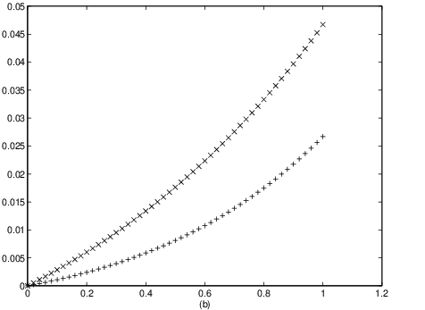
The result is shown in Figure ??(a). It can be seen that, indeed, we have obtained an upper bound for the global discretization error in (??). In the proof of part (c) of Proposition ?? we have used the fact that this upper bound tends to zero with decreasing step size $h$ . This fact is illustrated in Figure ??(b), where we have changed the step size 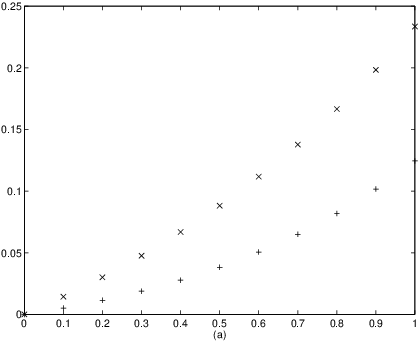$h$ to $0.02$ .

Figure 1: Comparison of the global discretization error (marked by $+$ ) with its estimate given in (??) (marked by $\times$ ) for the step sizes (a) $h=0.1$ and (b) $h=0.02$ .

Explicit Computation of Error Bounds

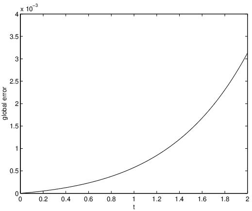
Another important consequence of Proposition ?? is that it allows us to compute the solution of the initial value problem (??) on a given interval $[0,T]$ up to a prescribed accuracy. Indeed, we just have to use the estimate (??) on the global discretization error.

For an illustration of this fact suppose that we want to approximate a solution of (??) on the interval $t\in [0,2]$ where the maximal global discretization error is less than $0.01$ . It follows from (??) that this is certainly the case if the step size $h$ is chosen such that $e^2(e^2-1)\frac {h}{2} = 0.01,$ or, equivalently, $h = \frac {0.02}{e^2(e^2-1)} \approx 0.000424.$ Indeed, if this is the case then we find with (??) $|\epsilon (k)| \le e^2(e^{kh}-1)\frac {h}{2} \le e^2(e^2-1)\frac {h}{2} = 0.01.$ The result of the corresponding MATLAB computation of the global discretization error is shown in Figure ??.

Figure 2: The global discretization error for the solution of (??) on the interval $[0,2]$ with step size $h=0.000424$ .

Exercises

In Exercises ?? – ?? compute bounds on the local and global error for Euler’s method applied to the given initial value problem. Perform the same steps as in the treatment of the initial value problem (??) in the text.

$\frac {\dps dx}{\dps dt} = 3x,\quad x(0)=1$ .

$\frac {\dps dx}{\dps dt} = x,\quad x(0)=2$ .

$\frac {\dps dx}{\dps dt} = 3x,\quad x(0)=2$ .

Apply the implicit Euler method to the initial value problem (??). Then determine a formula for the local discretization error that is analogous to (??). Hint: Before proceeding as for Euler’s method solve for $x_{k+1}$ in (??) in this specific case.

In Exercises ?? – ?? determine a step size $h$ such that the global discretization error for the solution of (??) on the given interval using Euler’s method is less than the given absolute tolerance. Verify your results by a computation of the global discretization error using MATLAB.

Interval $[0,4]$ and absolute tolerance $2$ .

Interval $[0,5]$ and absolute tolerance $10$ .

Suppose that you want to solve (??) by Euler’s method with a fixed step size $h=0.005$ on the interval $[0,T]$ . How large can you choose $T$ so that the global discretization error does not exceed $0.05$ ? Confirm your result using MATLAB.