RLC Circuits

$\newenvironment {prompt}{}{} \newcommand {\Sec }[2]{\section {#1}} \newcommand {\trademark }[0]{{R\!\!\!\!\!\bigcirc }} \newcommand {\EXER }[0]{\section *{Exercises}} \newcommand {\CEXER }[0]{} \newcommand {\TEXER }[0]{} \newcommand {\R }[0]{\mbox {$\Bbb {R}$}} \newcommand {\C }[0]{\mbox {$\Bbb {C}$}} \newcommand {\Z }[0]{\mbox {$\Bbb {Z}$}} \newcommand {\N }[0]{\mbox {$\Bbb {N}$}} \newcommand {\D }[0]{\mbox {{\bf D}}} \newcommand {\setmin }[0]{\;\mbox {--}\;} \newcommand {\Matlab }[0]{{M\small {AT\-LAB}} } \newcommand {\Matlabp }[0]{{M\small {AT\-LAB}}} \newcommand {\computer }[0]{\Matlab Instructions} \newcommand {\half }[0]{\mbox {$\frac {1}{2}$}} \newcommand {\compose }[0]{\raisebox {.15ex}{\mbox {{\scriptsize $\circ $}}}} \newcommand {\AND }[0]{\quad \mbox {and}\quad } \newcommand {\vect }[2]{\left (\begin {array}{c} #1_1 \\ \vdots \\ #1_{#2}\end {array}\right )} \newcommand {\mattwo }[4]{\left (\begin {array}{rr} #1 & #2\\ #3 &#4\end {array}\right )} \newcommand {\mattwoc }[4]{\left (\begin {array}{cc} #1 & #2\\ #3 &#4\end {array}\right )} \newcommand {\vectwo }[2]{\left (\begin {array}{r} #1 \\ #2\end {array}\right )} \newcommand {\vectwoc }[2]{\left (\begin {array}{c} #1 \\ #2\end {array}\right )} \newcommand {\inv }[0]{^{-1}} \newcommand {\CC }[0]{{\cal C}} \newcommand {\CCone }[0]{\CC ^1} \newcommand {\Span }[0]{{\rm span}} \newcommand {\rank }[0]{{\rm rank}} \newcommand {\trace }[0]{{\rm tr}} \newcommand {\RE }[0]{{\rm Re}} \newcommand {\IM }[0]{{\rm Im}} \newcommand {\nulls }[0]{{\rm null\;space}} \newcommand {\dps }[0]{\displaystyle } \newcommand {\arraystart }[0]{\renewcommand {\arraystretch }{1.8}} \newcommand {\arrayfinish }[0]{\renewcommand {\arraystretch }{1.2}} \newcommand {\Start }[1]{\vspace {0.08in}\noindent {\bf Section~\ref {#1}}} \newcommand {\exer }[1]{\noindent {\bf \ref {#1}}} \newcommand {\ans }[0]{} \newcommand {\matthree }[9]{\left (\begin {array}{rrr} #1 & #2 & #3 \\ #4 & #5 & #6 \\ #7 & #8 & #9\end {array}\right )} \newcommand {\cvectwo }[2]{\left (\begin {array}{c} #1 \\ #2\end {array}\right )} \newcommand {\cmatthree }[9]{\left (\begin {array}{ccc} #1 & #2 & #3 \\ #4 & #5 & #6 \\ #7 & #8 & #9\end {array}\right )} \newcommand {\vecthree }[3]{\left (\begin {array}{r} #1 \\ #2 \\ #3\end {array}\right )} \newcommand {\cvecthree }[3]{\left (\begin {array}{c} #1 \\ #2 \\ #3\end {array}\right )} \newcommand {\cmattwo }[4]{\left (\begin {array}{cc} #1 & #2\\ #3 &#4\end {array}\right )} \newcommand {\thehelp }[0]{\thesection .\arabic {equation}} \newcommand {\matlabEquation }[0]{\let \oldtheequation \theequation \renewcommand {\theequation }{\oldtheequation *}\begin {equation}} \newcommand {\HyperFirstAtBeginDocument }[0]{\AtBeginDocument } \newcommand {\epstopdfsetup }[0]{\setkeys {ETE}} changed the theorem header of amsthm failed\MessageBreak }}} \newcommand {\GetTitleStringSetup }[0]{\setkeys {gettitlestring}} \newcommand {\Sectionformat }[2]{#1}$ $% This file was *autogenerated* from rLCCircuits.sagetex.sage with % sagetex.py version 2015/08/26 v3.0-92d9f7a %f25d9a4bf01f4d6a708674cb562748c4% md5sum of corresponding .sage file (minus "goboom","current_tex_line",and pause/unpause lines)$

RLC circuits provide an excellent example of a physical system that is well modeled by a second order linear differential equation that is periodically forced by a discontinuous function. Consider the electrical circuit shown in Figure ??. The circuit consists of a resistor with resistance $R$ , a coil with inductance $L$ , a capacitor with capacitance $C$ , and a voltage source producing a time dependent voltage $V(t)$ .

Figure 1: An RLC circuit with resistance $R$ , inductance $L$ , capacitance $C$ , and a voltage source $V(t)$ .

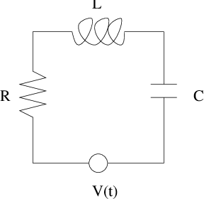
We describe the behavior of the circuit by the voltage drop $x(t)$ at the capacitor. Kirchhoff’s Laws for electric circuits show that $x(t)$ satisfies the second order differential equation

$\begin{equation} \label{e:eleccirc} \frac{1}{CL}V(t) = \frac{d^2x}{dt^2}(t) + \frac{R}{L}\frac{dx}{dt}(t) + \frac{1}{CL}x(t), \end{equation}$ as we now explain. Kirchhoff’s Voltage Law states that at each instant of time the voltage $V(t)$ produced at the source is equal to the sum of the voltage drops at the three elements of the circuit. So, if we denote the voltage drops at the coil by $V_{coil}$ and at the resistor by $V_{resistor}$ , then we have $\begin{equation} \label{e:kirchhoff} V(t) = V_{coil}(t) + V_{resistor}(t) + x(t), \end{equation}$ recalling that $x(t)$ is the voltage drop at the capacitor.

Let $I(t)$ be the current through the system. Then

The voltage drop in a capacitor is proportional to the charge difference $Q_{capacitor}$ between the two plates: $x(t) = \frac {1}{C}Q_{capacitor},$ where $C$ is the capacitance measured in farads. The charge difference itself is related to the current by $I = \frac {dQ_{capacitor}}{dt} = C\frac {dx}{dt}.$
The voltage drop at a resistor is proportional to the current: $V_{resistor} = RI = RC\frac {dx}{dt},$ where $R$ is the resistance measured in ohms.
The voltage drop in a coil is given by Faraday’s Law; the drop is proportional to the rate of change of the current: $V_{coil} = L\frac {dI}{dt} = LC\frac {d^2x}{dt^2},$ where $L$ is the inductance of the coil measured in henrys.

Combining (a,b,c) with (??), we obtain the differential equation: $V(t) = LC\ddot {x} + RC\dot {x} + x.$ After dividing by $LC$ , we obtain the second order equation (??); and, on setting $a = \frac {R}{L}, \quad b = \frac {1}{CL}, \AND g(t) = \frac {1}{CL}V(t),$ we have an initial value problem in the form (??).

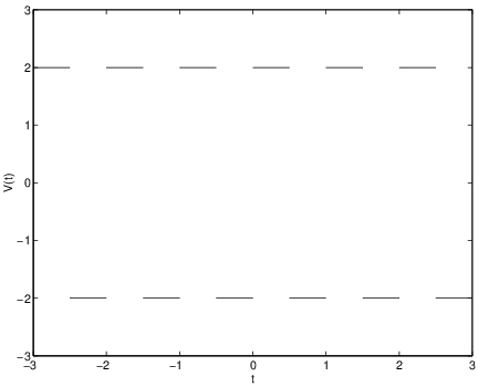
A typical input at the voltage source (associated to alternating current) is a $2T$ -periodic square wave with amplitude $A>0$ defined by periodicity and $V(t) = \left \{\begin {array}{rl} A & 0<t\leq T\\ -A & T<t\leq 2T. \end {array}\right .$ See Figure ??. We will see how to use Laplace transforms to solve second order equations with a discontinuous forcing of this type. Indeed, it is the possibility of using Laplace transforms to solve linear equations with piecewise smooth forcing terms that is the main strength of Laplace transforms.

Figure 2: A 1-periodic square wave $V(t)$ of amplitude $A=2$ .

Piecewise Smooth Periodic Forcing

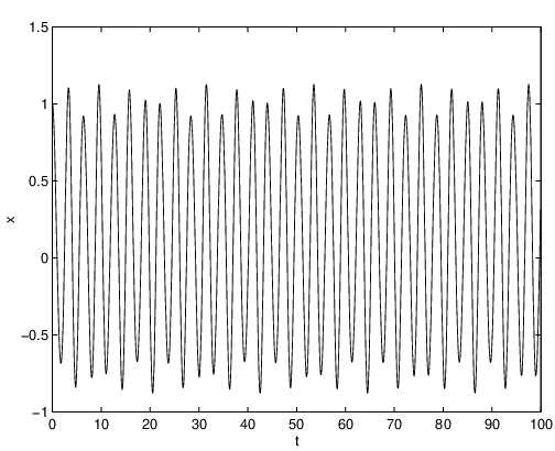
We now show how Laplace transforms can be used to solve second order equations with periodic discontinuous forcing. As an example we consider the equation (??) where the external force $g(t)$ is given by

$\begin{equation} g(t) = \left\{\begin{array}{cl} 1 & \mbox{for $t \in [2k,2k+1]$} \\ 0 & \mbox{for $t \in [2k+1,2k+2]$} \end{array} \right. (k=0,1,2,\ldots). \end{equation}$ We begin by computing the Laplace transform of $g(t)$ . Using the definition we obtain

$\begin{eqnarray*} {\cal L}[g] & = & \int_0^\infty e^{-st} g(t)\, dt\\ &=& \sum_{k=0}^\infty \int_k^{k+1} e^{-st} g(t)\, dt\\ &=& \sum_{k=0}^\infty \int_{2k}^{2k+1} e^{-st}\, dt, \end{eqnarray*}$

since $g(t)$ vanishes for $t \in [2k+1,2k+2]$ . Performing the integrations leads to

$\begin{eqnarray*} {\cal L}[g] & = & \frac{1}{s}\sum_{k=0}^\infty \left(e^{-2sk}-e^{-s(2k+1)}\right)\\ &=& \frac{1}{s}\sum_{k=0}^\infty (1-e^{-s})e^{-2sk}\\ &=& \frac{1}{s} (1-e^{-s}) \frac{1}{1-e^{-2s}}\\ &=& \frac{1}{s(1+e^{-s})}. \end{eqnarray*}$

Hence an application of the Laplace transform to the differential equation (??) gives $s^2{\cal L}[x]-s + 4{\cal L}[x] = {\cal L}[g] = \frac {1}{s(1+e^{-s})},$ and solving this for ${\cal L}[x]$ leads to ${\cal L}[x] = \frac {1}{s(s^2 +4)(1+e^{-s})} + \frac {s}{s^2 +4}.$ It remains to compute the inverse Laplace transform of the first term. For this we observe that for real numbers $x$ with $|x|<1$ the following identity holds: $\frac {1}{1+x} = 1-x+x^2-x^3+x^4-\cdots = \sum _{k=0}^\infty (-1)^k x^k.$ Hence, for positive $s$ , $\frac {1}{1+e^{-s}} = \sum _{k=0}^\infty (-1)^k e^{-sk},$ and it follows that

$\begin{eqnarray*} {\cal L}[x] &=&\frac{1}{s(s^2 +4)}\sum_{k=0}^\infty (-1)^k e^{-sk} + \frac{s}{s^2 +4}\\ &=& \frac{1}{4}\left(\frac{1}{s}-\frac{s}{s^2+4}\right) \sum_{k=0}^\infty (-1)^k e^{-sk} + \frac{s}{s^2 +4}\\ &=& \frac{1}{4}\left(\frac{1}{s}+\frac{3s}{s^2+4}+ \left(\frac{1}{s}-\frac{s}{s^2+4}\right) \sum_{k=1}^\infty (-1)^k e^{-sk}\right)\\ &=& \frac{1}{4}\left(\frac{1}{s}+\frac{3s}{s^2+4}+ \sum_{k=1}^\infty (-1)^k \frac{e^{-sk}}{s}- \sum_{k=1}^\infty (-1)^k \frac{e^{-sk}s}{s^2+4}\right). \end{eqnarray*}$

Now we have derived an expression for ${\cal L}[x]$ in which we can compute the inverse Laplace transform for each of the individual summands. Using Table ?? and Proposition ?? we obtain

$\begin{eqnarray*} x(t)&=&\frac{1}{4}\left(1+3\cos(2t)+\sum_{k=1}^\infty (-1)^k H_k(t) -\sum_{k=1}^\infty (-1)^k H_k(t)\cos(2(t-k))\right)\\ &=&\frac{1}{4}\left(1+3\cos(2t)+\sum_{k=1}^\infty (-1)^k H_k(t)(1-\cos(2(t-k)))\right)\\ &=&\frac{1}{4}\left(1+3\cos(2t)+2\sum_{k=1}^\infty (-1)^k H_k(t)\sin^2(t-k))\right). \end{eqnarray*}$

In Figure ?? we show the solution for $t\in [0,20]$ . Observe that this solution is certainly not periodic in time. Indeed, since the internal frequency of equation (??) is $1/\pi$ and the frequency of the external periodic forcing is $1/2$ we expect to obtain a quasiperiodic motion.

Figure 3: The solution of the initial value problem (??) where the external force is given by a periodic discontinuous function.