Level sets

$\newenvironment {prompt}{}{} \newcommand {\ungraded }[0]{} \newcommand {\todo }[0]{} \newcommand {\oiint }[0]{{\large \bigcirc }\kern -1.56em\iint } \newcommand {\mooculus }[0]{\textsf {\textbf {MOOC}\textnormal {\textsf {ULUS}}}} \newcommand {\npnoround }[0]{\nprounddigits {-1}} \newcommand {\npnoroundexp }[0]{\nproundexpdigits {-1}} \newcommand {\npunitcommand }[1]{\ensuremath {\mathrm {#1}}} \newcommand {\RR }[0]{\mathbb R} \newcommand {\R }[0]{\mathbb R} \newcommand {\N }[0]{\mathbb N} \newcommand {\Z }[0]{\mathbb Z} \newcommand {\sagemath }[0]{\textsf {SageMath}} \newcommand {\d }[0]{\,d} \newcommand {\l }[0]{\ell } \newcommand {\ddx }[0]{\frac {d}{\d x}} \newcommand {\zeroOverZero }[0]{\ensuremath {\boldsymbol {\tfrac {0}{0}}}} \newcommand {\inftyOverInfty }[0]{\ensuremath {\boldsymbol {\tfrac {\infty }{\infty }}}} \newcommand {\zeroOverInfty }[0]{\ensuremath {\boldsymbol {\tfrac {0}{\infty }}}} \newcommand {\zeroTimesInfty }[0]{\ensuremath {\small \boldsymbol {0\cdot \infty }}} \newcommand {\inftyMinusInfty }[0]{\ensuremath {\small \boldsymbol {\infty -\infty }}} \newcommand {\oneToInfty }[0]{\ensuremath {\boldsymbol {1^\infty }}} \newcommand {\zeroToZero }[0]{\ensuremath {\boldsymbol {0^0}}} \newcommand {\inftyToZero }[0]{\ensuremath {\boldsymbol {\infty ^0}}} \newcommand {\numOverZero }[0]{\ensuremath {\boldsymbol {\tfrac {\#}{0}}}} \newcommand {\dfn }[0]{\textbf } \newcommand {\unit }[0]{\mathop {}\!\mathrm } \newcommand {\eval }[1]{\bigg [ #1 \bigg ]} \newcommand {\seq }[1]{\left ( #1 \right )} \newcommand {\epsilon }[0]{\varepsilon } \newcommand {\phi }[0]{\varphi } \newcommand {\iff }[0]{\Leftrightarrow } \DeclareMathOperator {\arccot }{arccot} \DeclareMathOperator {\arcsec }{arcsec} \DeclareMathOperator {\arccsc }{arccsc} \DeclareMathOperator {\si }{Si} \DeclareMathOperator {\scal }{scal} \DeclareMathOperator {\sign }{sign} \newcommand {\arrowvec }[1]{{\overset {\rightharpoonup }{#1}}} \newcommand {\vec }[1]{{\overset {\boldsymbol {\rightharpoonup }}{\mathbf {#1}}}\hspace {0in}} \newcommand {\point }[1]{\left (#1\right )} \newcommand {\pt }[1]{\mathbf {#1}} \newcommand {\Lim }[2]{\lim _{\point {#1} \to \point {#2}}} \DeclareMathOperator {\proj }{\mathbf {proj}} \newcommand {\veci }[0]{{\boldsymbol {\hat {\imath }}}} \newcommand {\vecj }[0]{{\boldsymbol {\hat {\jmath }}}} \newcommand {\veck }[0]{{\boldsymbol {\hat {k}}}} \newcommand {\vecl }[0]{\vec {\boldsymbol {\l }}} \newcommand {\uvec }[1]{\mathbf {\hat {#1}}} \newcommand {\utan }[0]{\mathbf {\hat {t}}} \newcommand {\unormal }[0]{\mathbf {\hat {n}}} \newcommand {\ubinormal }[0]{\mathbf {\hat {b}}} \newcommand {\dotp }[0]{\bullet } \newcommand {\cross }[0]{\boldsymbol \times } \newcommand {\grad }[0]{\boldsymbol \nabla } \newcommand {\divergence }[0]{\grad \dotp } \newcommand {\curl }[0]{\grad \cross } \newcommand {\lto }[0]{\mathop {\longrightarrow \,}\limits } \newcommand {\bar }[0]{\overline } \newcommand {\surfaceColor }[0]{violet} \newcommand {\surfaceColorTwo }[0]{redyellow} \newcommand {\sliceColor }[0]{greenyellow} \newcommand {\vector }[1]{\left \langle #1\right \rangle } \newcommand {\sectionOutcomes }[0]{} \newcommand {\HyperFirstAtBeginDocument }[0]{\AtBeginDocument }$

We introduce level sets.

Level sets

It was Descartes who said “Je pense, donc je suis”. He also developed our rectangular coordinate system, the $(x,y)$ -plane. This is also known as the Cartesian coordinate system. This coordinate system allows us to consider the graph of a function. First, recall that the graph of a function of a single variable, $y=f(x)$ is a curve in a two-dimensional plane. In the same sense, the graph of a function of two variables, $z = F(x,y)$ is a surface in three-dimensional space. The graph of a function of three variables, $w=F(x,y,z)$ is a surface in four-dimensional space. A surface in higher than three dimensions is often called a hypersurface. How can we visualize such functions? For visualizing functions $f:\R \to \R$ , a graphing utility like Desmos is really great. For visualizing functions $F:\R ^2\to \R$ , GeoGebra is very helpful. However, once we get to functions $F:\R ^3\to \R$ (or $F: \R ^n \to \R$ ), visualizing the graph of the function as we do in two and three dimensions becomes much more difficult. One powerful technique to help us understand a function $F:\R ^3\to \R$ visually is known as sketching level sets.

Suppose that $F:\R ^n \to \R$ is a function and $c$ is in the range of $F$ . A level set corresponding to an output $c$ is a set of all points $\vec {x}$ in the domain of $F$ with the property that $F(\vec {x}) = c$ .

(In other words, all the points in the level set are assigned the same value, $c$ , by the function $F$ , and any point in the domain of $F$ with output $c$ is in that level set .)

When working with functions $F:\R ^2\to \R$ , the level sets are known as level curves.

When we are looking at level curves, we can think about choosing a $z$ -value, say $z=c$ , in the range of the function and ask “at which points $(x,y)$ can we evaluate the function to get $F(x,y)=c$ ?” Those points form our level curve. If we choose a value $z=c$ that was not in the range of $F$ , there would be no points in the $(x,y)$ -plane for which $F(x,y)=c$ , and hence no level curve associated to $z = c$ .

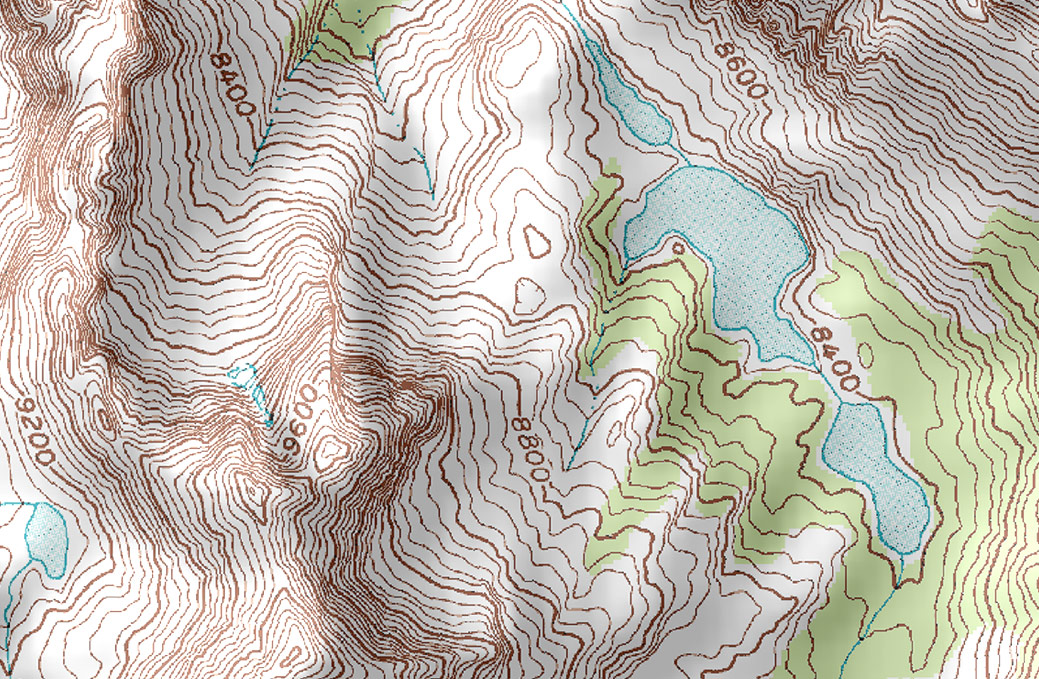
It may be surprising to find that the concept of level sets is familiar to most people, but they don’t realize it. Topographical maps, like the one below represent the surface of Earth by indicating points with the same elevation with contour lines. We also had an example of the contour lines of Meteor Crater as we began this section.

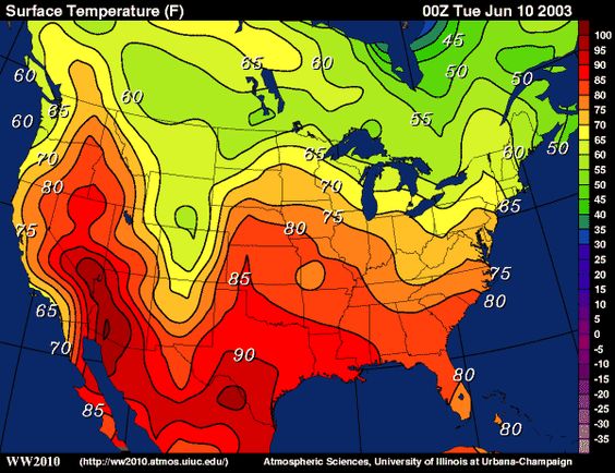
Another example you may know are isotherms, which are curves along which the temperature does not change. We see these in weather maps.

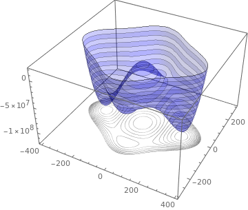
Below we see a surface with level curves drawn beneath the surface. Remember that the level curves are in the domain of the function, not on the surface itself.

Given that $z=c$ is in the range of $z=F(x,y)$ , select the statements below that are true.

The level curves $F(x,y)=c$ are in the domain of the function. The level curves $F(x,y)=c$ are in the $(x,y)$ -plane. The level curves $F(x,y)=c$ are in the range of the function. The level curves $F(x,y)=c$ are on the surface $z=F(x,y)$ . The level curves $F(x,y)=c$ can also be thought of as the intersection of the plane $z=c$ with the surface $z=F(x,y)$ .

We often mark the function value on the corresponding level set. If we choose function values which have a constant difference, then level curves are close together when the function values are changing rapidly, and far apart when the function values are changing slowly.

Suppose you have a differentiable function $F:\R ^2\to \R$ with the following set of level curves. You should interpolate reasonable values of the function $F$ between the level curves which are shown:

Consider the points $A$ , $B$ , and $C$ on the surface $z=F(x,y)$ . Order the points from least steep to most steep.

At point $\answer [format=string]{C}$ the surface is less steep than at point $\answer [format=string]{A}$ , and the surface is steepest at point $\answer [format=string]{B}$ .

Since the $z$ -values on the level curves are equally spaced in this example, level curves which are close together indicate more rapid change in the $z$ -values, while level curves which are further apart indicate slower change in the $z$ -values.

Now, let’s see if you can identify some simple surfaces based on their level curves.

Match the following level sets to the equations below.

$\begin{align*} &\answer[format=string]{D}: x+z=3\\ &\answer[format=string]{C}: y+z=-2\\ &\answer[format=string]{B}: x+y+z=-3\\ &\answer[format=string]{A}: -x+y+z=2 \end{align*}$

Let’s look at another example.

Suppose that $F(x,y) = x^2-y^2$ . Sketch the level curves of $F$ for $c=-3$ , $-2$ , $-1$ , $0$ , $1$ , $2$ , and $3$ .

First, notice that the domain of $F$ is $\R ^2$ , and the range of $F$ is $\R$ . It’s particularly important to notice that all of the values of $c$ we will use to find level curves are in the range of $F$ .

Now let’s find the level curves of $F$ for the required values. Each of our level curves will be of the form $c = \answer [given]{x^2-y^2}$ Now we just need to substitute all of our values for $c$ and plot each of the following implicit functions:

$\begin{align*} -3 &= x^2-y^2\\ -2 &= x^2-y^2\\ -1 &= x^2-y^2\\ 0 &= x^2-y^2\\ 1 &= x^2-y^2\\ 2 &= x^2-y^2\\ 3 &= x^2-y^2 \end{align*}$ To make your sketch, either plot these implicit functions with your favorite graphing device, or recognize that they are crossing lines when $x=y=0$ and hyperbolas otherwise. As a gesture of friendship, we have included a graph of these level curves. $\graph [xmin=-5, xmax=5, ymin=-2.5, ymax=2.5]{-3=x^2-y^2,-2=x^2-y^2,-1=x^2-y^2,0=x^2-y^2,1=x^2-y^2,2=x^2-y^2,3=x^2-y^2}$ Below, we evaluate $F$ on our level curves and plot the resulting curves on the surface $F$ .

Notice how the difference between consecutive $c$ values is always $1$ , so we can use the closeness of the level curves on the $(x,y)$ -plane to determine how the surface is changing. Near the level curves of $c=0$ and $c=1$ we can both predict (from our sketch of just the level curves) as well as see (on our graph of the curves on the surface) that $F$ indeed is growing quickly.

Let’s see another example.

Suppose that $F(x,y) = 4xy+3y^2+3$ . Find the equation of the level curve that passes through $(x,y) = (1,2)$ in terms of $x$ and $y$ , and then find a parametric description for both the level curve as well as the corresponding curve on the surface.

First, find the equation of the level curve. Note that the level curve consists of all points in the $(x,y)$ -plane that give the same value for $F(x,y)$ . Since $(1,2)$ lies on this curve, and $F(1,2) = \answer [given]{23}$ , the equation of the level curve is $4xy+3y^2+3 = \answer [given]{23}$ , or $4xy+3y^2 = \answer [given]{20}$ .

Now, we find a vector-valued function for the level curve, as well as the curve on the surface. Since the level curve is given by the equation $4xy+3y^2 = 20$ and we can solve for $x$ without too much algebra, we set $y=t$ . Then, $x =\answer [given]{\frac {20-3t^2}{4t}}$ . The level curve can be described parametrically by: $\vec {p} (t) = \vector {\answer [given]{\frac {20-3t^2}{4t}}, \answer [given]{t}}$ The corresponding curve on the surface can be described parametrically by:

$\begin{align*} \vec{r} (t) &= \vector{\answer[given]{(20 - 3 t^2)/(4 t)},\answer[given]{t},F\left(\vec{p}(t) \right)} \\ &= \vector{\answer[given]{\frac{20-3t^2}{4t}}, \answer[given]{t}, \answer[given]{23}} \end{align*}$

Notice that the $z$ -component of the curve on the surface should not require much calculation since we found the curve on the surface by noting $F(1,2) =23$ . This means that all of the $z$ -values on the curve on the surface should be $\answer [given]{23}$ .

So far, the level sets we’ve been working with have been curves in $\R ^2$ . We can easily generalize to functions $F:\R ^n \to \R$ . When working with functions $F:\R ^3\to \R$ , our level sets are also called level surfaces.

Level sets in higher dimensions

In higher dimensions, we use what we understand about functions of one and two variables to try to better understand functions of three or more variables.

A function of one variable can be visualized as a curve drawn in two dimensions.
A function of two variables can be visualized as a surface drawn in three dimensions.
A function of three variables can be visualized as what we will call a hypersurface drawn in four dimensions.
A function of $n$ variables can be visualized as what we will call a hypersurface drawn in $n+1$ dimensions.

We use the term “hypersurface” to refer to an object which is like a surface, but in more than three dimensions. Hypersurfaces are difficult to imagine, and can even be difficult to picture using modern computer utilities.

For a function $F: \R ^3 \to R$ of three variables, one technique we can use is to graph the level surfaces, our three-dimensional analogs of level curves in two dimensions. Given $w=F(x,y,z)$ , the level surface at $w=c$ is the surface in space formed by all points $(x,y,z)$ where $F(x,y,z)=c$ . It’s time for an example.

If a point source $S$ is radiating energy, the intensity $I$ at a given point $P$ in space is inversely proportional to the square of the distance between $S$ and $P$ . That is, when $S=(0,0,0)$ , $\begin{align*} I(x,y,z) &= \frac{\text{some constant}}{\text{distance squared}}\\ &=\frac{k}{x^2+y^2+z^2} \end{align*}$ for some constant $k$ . Let $k=1$ ; find the level surfaces of $I$ .

First, let’s think about this situation. If energy (say, in the form of light) is emanating from the origin, its intensity will be the same all a points equidistant from the origin. That is, at any point on the surface of a sphere centered at the origin, the intensity should be the same. Therefore, the level surfaces must be spheres.

We now confirm our thought process mathematically. The level surface at $I=c$ , where $c>0$ , is defined by $c = \frac {1}{x^2+y^2+z^2}.$ Algebra reveals $\answer [given]{x^2+y^2+z^2} = \frac {1}{c}.$ Given an intensity $c$ , the level surface $I=c$ is a sphere of radius $1/\sqrt {c}$ , centered at the origin. Every point on each sphere experiences the same intensity of the radiating energy.

We have found that the level surfaces of $F$ in the above example are concentric spheres. If we picture several of these concentric spheres at the same time, we can get some intuition about the graph of $F$ in four dimensions in the same way that a collection of level curves in two dimensions gave us some intuition about the corresponding surface in three dimensions.

From explicit surfaces to level surfaces

We turn our attention to an important concept that will arise again in future sections.

Suppose that $F:\R ^2 \to \R$ is a function of two variables. Then, the graph of $F$ , i.e., the surface $z = F(x,y)$ is a level surface of the function $G(x,y,z) = F(x,y) - z.$

In fact, if $F: \R ^n \to \R$ is a function of $n$ variables, we can also consider it to be a particular level set for some other function $G: \R ^{n+1} \to \R$ of $n+1$ variables. This idea is very powerful, as it allows us to consider the same surface from two different perspectives. Having multiple perspectives gives us extra tools to use when considering our surface, as well as allows us to look at the surface in whatever manner we find most convenient. Let’s consider a specific example.

Suppose that $z=x^2+y-3$ . Find a function $G:\R ^3\to \R$ such that $z=x^2+y-3$ is a level surface of $G$ .

We can move $z$ to the right-hand side to obtain: $0 = \answer [given]{x^2+y-3-z}$ We can now set $G(x,y,z) = x^2+y-3-z$ and recognize that our original surface is the level surface of $G(x,y,z) = x^2+y-3-z$ corresponding to output $0$ .

Therefore, the surface can be interpreted as the graph of $F$ , where $F$ is a function of two variables given by $F(x,y) = x^2+y-3$ or as a level surface of $G$ , where $G$ is a function of three variables, given by $G(x,y,z)=x^2+y-3-z$ . To summarize, the following two equations describe the same surface $z=F(x,y)$ or $G(x,y,z)=0$

Again, it appears that all we did here was some easy algebra. We made a new function of one more variable by simply rearranging the original equation that defined our surface. But having multiple perspectives is always better than having only one. In addition to its other uses, the content of this procedure is vital for

finding normal vectors for explicitly defined surfaces.
finding tangent planes for explicitly defined surfaces.

These results will be explored further in later sections. It’s good to become familiar with these ideas now, so that we can make expert use of them later.