Functions of several variables

$\newenvironment {prompt}{}{} \newcommand {\ungraded }[0]{} \newcommand {\todo }[0]{} \newcommand {\oiint }[0]{{\large \bigcirc }\kern -1.56em\iint } \newcommand {\mooculus }[0]{\textsf {\textbf {MOOC}\textnormal {\textsf {ULUS}}}} \newcommand {\npnoround }[0]{\nprounddigits {-1}} \newcommand {\npnoroundexp }[0]{\nproundexpdigits {-1}} \newcommand {\npunitcommand }[1]{\ensuremath {\mathrm {#1}}} \newcommand {\RR }[0]{\mathbb R} \newcommand {\R }[0]{\mathbb R} \newcommand {\N }[0]{\mathbb N} \newcommand {\Z }[0]{\mathbb Z} \newcommand {\sagemath }[0]{\textsf {SageMath}} \newcommand {\d }[0]{\,d} \newcommand {\l }[0]{\ell } \newcommand {\ddx }[0]{\frac {d}{\d x}} \newcommand {\zeroOverZero }[0]{\ensuremath {\boldsymbol {\tfrac {0}{0}}}} \newcommand {\inftyOverInfty }[0]{\ensuremath {\boldsymbol {\tfrac {\infty }{\infty }}}} \newcommand {\zeroOverInfty }[0]{\ensuremath {\boldsymbol {\tfrac {0}{\infty }}}} \newcommand {\zeroTimesInfty }[0]{\ensuremath {\small \boldsymbol {0\cdot \infty }}} \newcommand {\inftyMinusInfty }[0]{\ensuremath {\small \boldsymbol {\infty -\infty }}} \newcommand {\oneToInfty }[0]{\ensuremath {\boldsymbol {1^\infty }}} \newcommand {\zeroToZero }[0]{\ensuremath {\boldsymbol {0^0}}} \newcommand {\inftyToZero }[0]{\ensuremath {\boldsymbol {\infty ^0}}} \newcommand {\numOverZero }[0]{\ensuremath {\boldsymbol {\tfrac {\#}{0}}}} \newcommand {\dfn }[0]{\textbf } \newcommand {\unit }[0]{\mathop {}\!\mathrm } \newcommand {\eval }[1]{\bigg [ #1 \bigg ]} \newcommand {\seq }[1]{\left ( #1 \right )} \newcommand {\epsilon }[0]{\varepsilon } \newcommand {\phi }[0]{\varphi } \newcommand {\iff }[0]{\Leftrightarrow } \DeclareMathOperator {\arccot }{arccot} \DeclareMathOperator {\arcsec }{arcsec} \DeclareMathOperator {\arccsc }{arccsc} \DeclareMathOperator {\si }{Si} \DeclareMathOperator {\scal }{scal} \DeclareMathOperator {\sign }{sign} \newcommand {\arrowvec }[1]{{\overset {\rightharpoonup }{#1}}} \newcommand {\vec }[1]{{\overset {\boldsymbol {\rightharpoonup }}{\mathbf {#1}}}\hspace {0in}} \newcommand {\point }[1]{\left (#1\right )} \newcommand {\pt }[1]{\mathbf {#1}} \newcommand {\Lim }[2]{\lim _{\point {#1} \to \point {#2}}} \DeclareMathOperator {\proj }{\mathbf {proj}} \newcommand {\veci }[0]{{\boldsymbol {\hat {\imath }}}} \newcommand {\vecj }[0]{{\boldsymbol {\hat {\jmath }}}} \newcommand {\veck }[0]{{\boldsymbol {\hat {k}}}} \newcommand {\vecl }[0]{\vec {\boldsymbol {\l }}} \newcommand {\uvec }[1]{\mathbf {\hat {#1}}} \newcommand {\utan }[0]{\mathbf {\hat {t}}} \newcommand {\unormal }[0]{\mathbf {\hat {n}}} \newcommand {\ubinormal }[0]{\mathbf {\hat {b}}} \newcommand {\dotp }[0]{\bullet } \newcommand {\cross }[0]{\boldsymbol \times } \newcommand {\grad }[0]{\boldsymbol \nabla } \newcommand {\divergence }[0]{\grad \dotp } \newcommand {\curl }[0]{\grad \cross } \newcommand {\lto }[0]{\mathop {\longrightarrow \,}\limits } \newcommand {\bar }[0]{\overline } \newcommand {\surfaceColor }[0]{violet} \newcommand {\surfaceColorTwo }[0]{redyellow} \newcommand {\sliceColor }[0]{greenyellow} \newcommand {\vector }[1]{\left \langle #1\right \rangle } \newcommand {\sectionOutcomes }[0]{} \newcommand {\HyperFirstAtBeginDocument }[0]{\AtBeginDocument }$

We introduce functions that take vectors or points as inputs and output a number.

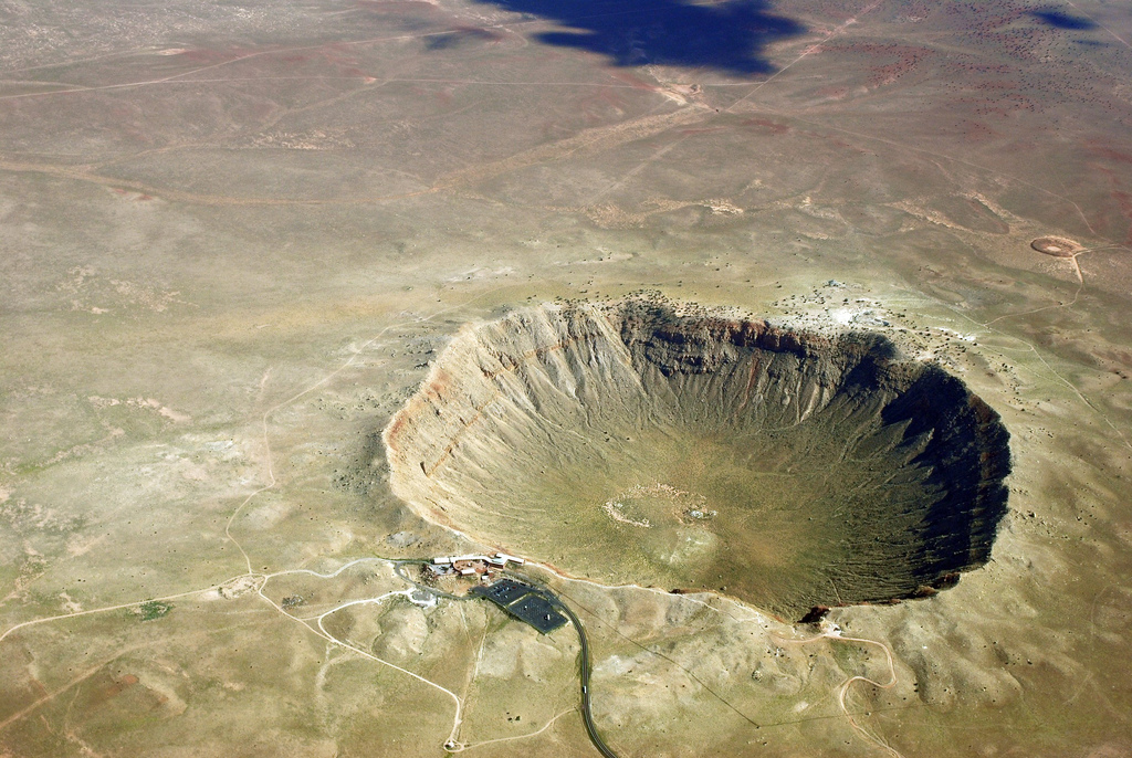
The world is constantly changing. Sometimes this change is very slow, other times it is shockingly fast. Consider Meteor Crater in northern Arizona.

This area was once grasslands and woodlands inhabited by bison, camels, wooly mammoths, and giant ground sloths. During the Pleistocene epoch, a meteor only $40$ meters in diameter collided with the Earth and this changed very quickly. The collision released around $4\times 10^{16}$ joules of energy, comparable to the energy released by a large nuclear weapon. A fireball extended out $10$ kilometers from the center of the impact, destroying all life in its wake. It is estimated it took one hundred years for the local plant and animal life to repopulate the area. Fifty thousand years later, the remains of the impact crater are still intact on our ever-changing Earth.

To help us understand events like these, we need to precisely describe what we are observing (in this case, the crater). To do this we use a contour map, often called a topographical map:

In essence, we are looking at the crater from directly above, and each curve in the map above represents a fixed, constant height. Mathematically, a contour map illustrates a function of two variables. We will now define a more general case of a function of $n$ variables. These are often called functions of several variables.

Let $D$ be a subset of $\R ^n$ . A function $F$ of $n$ variables, also called a function $F$ of several variables, with domain $D$ is a relation that assigns to every ordered $n$ -tuple in $D$ a unique real number in $\R$ . We denote this by each of the following types of notation. $\begin{align*} F: D &\to \R\\ \pt{x} &\mapsto y\\ \point{x_1,x_2,\dots,x_n} &\mapsto y\\ \vec{x} &\mapsto y\\ \vector{x_1,x_2,\dots,x_n} &\mapsto y\\ \end{align*}$

The range of $F$ is the set of all outputs of $F$ . It is a subset of $\R$ , not $\R ^n$ .

Consider $\begin{align*} F: \R^2 &\to \R\\ (x,y) &\mapsto x^2+y^2. \end{align*}$ Find the domain and range of $F$ .

Here, the domain is $(-\infty ,\infty )$ $\R ^2$ $\R ^n$ All points $(x,y)$ in $\R ^2$ with $x \geq 0$ and $y \geq 0$ and the range is $(-\infty ,\infty )$ $[0,\infty )$ $\R ^2$ $\R ^n$ .

The relationship from the previous example can be described more succinctly by the equation $F(x,y)=x^2+y^2,$ which is the notation that we will use most frequently when describing functions.

In this text, we will use an upper-case letter to denote a function of several variables.

Often, we will not specify the domain of a function in order to shorten its description. Unless otherwise specified, we will take the domain of a given function on $\R ^n$ to be the set of all ordered $n$ -tuples in $\R ^n$ for which the given expression is defined. We are familiar with this concept from one-variable calculus, where we would see a function defined by a formula such as $f(x) = \sqrt {x}$ and take its domain to be $[0, \infty )$ . In our example $F(x,y) = x^2+y^2$ , we take its domain to be $\R ^2$ .

Let’s investigate a few functions of two variables, $F:\R ^2\to \R$ .

Consider $F(x,y) = \ln (9-x^2-y^2).$ What is $F(2,1)$ ? $F(2,1) = \answer {\ln (4)}$

What is the domain of $F$ ?

Since we have not specified the domain, we take it to be the set of all vectors $\point {x,y}$ allowable as for $F$ . Because of the logarithm, we need $\point {x,y}$ such that $0 < 9-x^2-y^2$ $0 \leq 9-x^2-y^2$ $0 > 9-x^2-y^2$ $0 \geq 9-x^2-y^2$

The observant reader may note that this inequality describes the interior of a circle of radius $\answer [given]{3}$ centered at $(0,0)$ in the $(x,y)$ -plane, since we can write

$\begin{align*} 0 & < 9-x^2-y^2 \\ \answer{x^2+y^2} &< 9. \end{align*}$ While the domain may not always be easy to visualize, it is excellent practice and often insightful to try such a visualization.

What is the range of $F$ ?

The range is the set of all possible values. If we visualize the graph of $y = \ln (x)$ , we can see that the logarithm function outputs all values in $(-\infty , \infty )$ . However, the input for our logarithm function is not any value of $x$ , but any value of $9 - x^2 - y^2$ . Since the $x$ and $y$ terms are squared and then subtracted from $9$ , the largest possible value of $9-x^2-y^2$ occurs where $x=\answer {0}$ and $y=\answer {0}$ , in which case $F(0,0) = \answer {\ln (9)}$ . Notice that we must also have $9-x^2-y^2 > \answer [given]{0}$ in order to calculate the logarithm.

What do these calculations mean for the range of $F$ ?

In general, the logarithm is an function of its input, meaning that as the input gets larger, the output gets . In other words, the largest value of $9-x^2-y^2$ gives us the largest possible value of $F$ . We similarly find smaller values of $F$ by plugging in smaller values of $9-x^2-y^2$ . We have determined that the values of $9-x^2-y^2$ which make sense for this problem are those in the interval $(0, 9]$ , and so evaluating the logarithm on this interval gives us that the range $R$ is the interval $\left (\answer {-\infty },\answer {\ln (9)}\right ]$ .

Consider this geometric example.

The volume of a cylinder with base radius $R$ and height $h$ is given by $V=\pi R^2h.$ We can now think of the volume of a cylinder as a function of two variables, $R$ and $h$ $V(R,h) = \pi R^2h.$ Find the domain and the range of $V$ .

By requiring that the radius and height be nonnegative, we find that the domain is $\R$ $[0,\infty )$ Points $(R,h)$ in $\R ^2$ where $R \geq 0$ and $h \geq 0$ , or in set notation $\{ (R,h) \in \R ^2 : R \geq 0, h \geq 0\}$ . The range is: $\R$ $[0,\infty )$ $\{ (R,h) \in \R ^2 : R \geq 0, h \geq 0\}$ . The domain represents the set of all possible nonnegative radii and heights of the cylinder, and the range represents the set of all possible volumes that a cylinder could have.

Visualizing functions of several variables

There are many ways to interpret a function of several variables. Two very common ways to do this are to consider the surface obtained by graphing the function or to look at what we will call the level sets of our function.

Recall that given a function $f(x)$ of a single variable, we can consider the equation $y=f(x)$ , which allows us to visualize the function as the set of all points $(x,y)$ in the $(x,y)$ -plane. To do this, we pick an $x$ -value in the domain, and then the corresponding $y$ -coordinate is given by $f(x)$ .

Given a function $F(x,y)$ of two variables, we can take the same approach. We’ll consider the set of all points in $(x,y,z)$ -space where $z=F(x,y)$ . By choosing a point $(x,y)$ in the domain of the function, the corresponding $z$ -coordinate will be given by $F(x,y)$ .

Thus, one way of visualizing the function $F(x,y)$ is to consider the equation $z=F(x,y)$ and consider the set of all of the points in the $(x,y,z)$ -space that satisfy this criteria. We can then interpret that the function assigns a height to each point $(x,y)$ in its domain. Be very careful with this way of visualizing the function, however! The “height” can sometimes be negative, while we tend to almost always visualize a positive height.

We do not always interpret the output $F(x,y)$ as a height. For instance, we might want to talk about a density function for a region in $\R ^2$ , and define a function $\rho (x,y)$ by the density at each point $(x,y)$ in the region. We can still graph $z=\rho (x,y)$ , but the $z$ -values now should be interpreted as densities. Be careful to keep the meaning of the function in mind.

To make a sketch of a surface, we can specify many locations in the $(x,y)$ -plane (by picking many different values for $x$ and $y$ ), and plot the corresponding $z$ -values. While this is tedious to do by hand, computers can do it very easily. For example, if we consider the function $F(x,y) = 2-4x^3+y^2$ , we can evaluate the function at many different points $(x,y)$ and plot the results. For instance, at the point $(x,y)=(1,2)$ , we have $F(1,2) = \answer [given]{2}$ . Using software to graph both the surface and this point gives the following.

Generating curves on surfaces

Recall that we described curves in $\R ^n$ by giving vector-valued functions $\vec {p}(t)$ , where the coordinates of any point on the curve can be determined from a single parameter. We would now like to consider vector-valued functions alongside functions of several variables. As usual, we will work with two variables so that we can better visualize our examples, but our results will also extend to the case of $n$ variables.

If we have a function $F(x,y) : D \to \R$ and a vector-valued function $\vec {p}(t) = \vector {x(t), y(t)}$ so that for any value of $t$ , $\point {x(t), y(t)}$ is in the domain $D$ , we can evaluate $F$ at each point along the curve $\vec {p}$ and produce another curve $F\left (\vec {p} \right )$ on the surface.

Consider again $F(x,y) = 2-x^3+y^2$ . Also consider the curve defined by $y=2x$ in the $(x,y)$ -plane. Note that the domain of $F(x,y) = 2-x^3+y^2$ is all of $\R ^2$ , so each point on $\vec {p}(t) = \vector {t, 2t}$ is in the domain of $F$ .

Fill out the table below: $\begin {array}{c|c||c|c||c} x & y =2x & (x,y) & z=2-x^3+y^2 & (x,y,z) \\ \hline -0.5 & -1 & \left (-0.5,-1\right ) &3.125 & \left (-0.5, -1,3.125\right )\\ 0 & \answer [given]{0} & \left (\answer [given]{0},\answer [given]{0}\right ) & \answer [given]{2} & \left (\answer [given]{0},\answer [given]{0}, \answer [given]{2}\right ) \\ 0.5 & \answer [given]{1} & \left (\answer [given]{0.5}, \answer [given]{1}\right ) & \answer [given]{2.875} & \left (\answer [given]{0.5}, \answer [given]{1}, \answer [given]{2.875}\right )\\ 1 & \answer [given]{2} & \left (\answer [given]{1},\answer [given]{2}\right ) & \answer [given]{5} & \left (\answer [given]{1}, \answer [given]{2}, \answer [given]{5}\right ) \end {array}$ The points $(x,y)$ in our table lie on the curve $\vec {p}(t) = \vector {t, 2t}$ in the $(x,y)$ -plane. The points $(x,y,z) = (x,y,F(x,y))$ in our table lie on the surface $z=F(x,y)$ . If we would evaluate $F\left (\vec {p}(t) \right )$ for every point on $\vec {p}(t)$ we would see the curve on the surface corresponding to the curve in the plane, as pictured below.

We can think of the function as “lifting” a curve onto the surface $z=F(x,y)$ in $(x,y,z)$ -space. Of course, the curve must be in the domain of the function $F$ , and we should always be cautious when using the notion of “height” for our $z$ -coordinate.

So far, we have focused mainly on the curve $\vec {p}(t)= \vector {x(t), y(t)}$ lying in the domain of a function $F$ . Let’s now focus on the curve $\vector {x(t), y(t), F \left ( \vec {p} (t) \right )}$ on the surface. Since the curve is in $\R ^n$ , we must use a parametric equation to describe it. Fortunately, with our background on vector-valued functions, finding such a description should be straightforward.

Let $F(x,y) = 2-x^3+y^2$ as before. Give a parametric description of the the curve $\vec {r}(t)$ that lies on the surface $z=F(x,y)$ above the line $y=2x$ in the $(x,y)$ -plane.

A parameterization $\vec {p}(t)$ of $y = 2x$ in the $(x,y)$ -plane is

$\vec {p}(t) = \vector {t, \answer [given]{2t}}.$

We can now use the equation of the surface $z=F(x,y)$ to give $z$ in terms of $t$ . Since $z=2-x^3+y^2$ , setting $x=t$ and expressing $y$ in terms of $t$ gives $z(t) = \answer [given]{2+4t^2-t^3}$ . Thus, a parameterization of the curve is $\vec {r}(t) =\point {\answer [given]{t} , \answer [given]{2t}, \answer [given]{2+4t^2-t^3}}.$

The idea of looking at a curve in the domain of $F$ and the corresponding curve on the graph of $F$ can be helpful when thinking about many topics that follow. We may see these ideas again when we discuss limits of functions of several variables, derivatives and differentiability, the chain rule, tangent planes, as well as constrained optimization. Any time we work with these curves on surfaces, remember to think carefully about whether we are working in the domain of $F$ or on the surface $z=F(x,y)$ itself.