Lagrange Multipliers

$\newenvironment {prompt}{}{} \newcommand {\DeclareMathOperator }[2]{\@OldDeclareMathOperator {##1}{##2}\immediate \write \myfile {\unexpanded {\DeclareMathOperator }{\unexpanded {##1}}{\unexpanded {##2}}}} \newcommand {\ungraded }[0]{} \newcommand {\reserved@a }[2]{} \newcommand {\HyperFirstAtBeginDocument }[0]{\AtBeginDocument } \newcommand {\reserved@a }[1]{} \newcommand {\reserved@a }[2]{} \newcommand {\vnameref }[1]{\unskip ~\nameref {##1}\@vpageref [\unskip ]{##1}} \newcommand {\ref }[0]{\@ifstar \@refstar \T@ref } \newcommand {\pageref }[0]{\@ifstar \@pagerefstar \T@pageref } \newcommand {\nameref }[0]{\@ifstar \@namerefstar \T@nameref } \newcommand {\reserved@a }[2]{} \newcommand {\reserved@a }[0]{\AtBeginDocument } \newcommand {\reserved@a }[1]{} \newcommand {\reserved@a }[2]{}$

We’ve seen how we can optimize a function subject to a constraint using substitution, and we’ve seen that it can be very difficult to correctly handle the constraints! Fortunately, there is a tool that we can use to simplify this process. This tool is called “Lagrange multipliers.”

Gradients

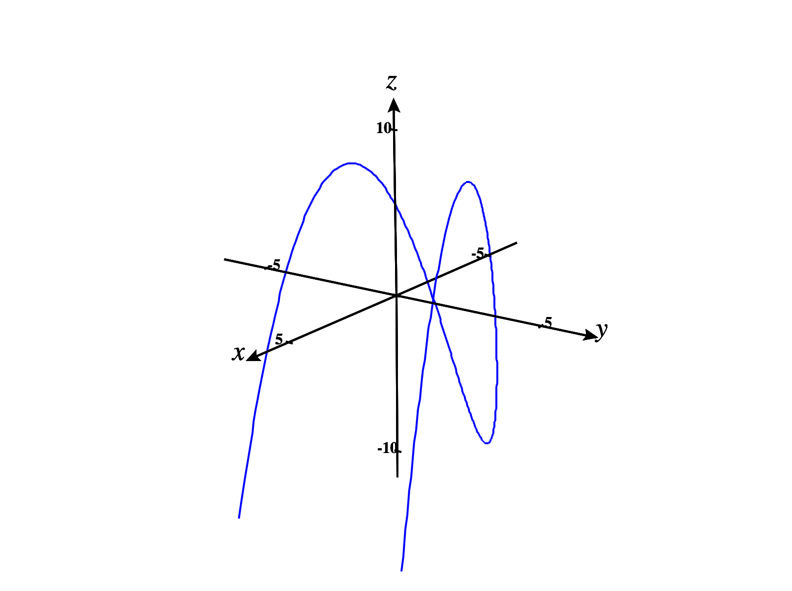
Suppose we wish to optimize a function $f:\mathbb {R}^n\rightarrow \mathbb {R}$ subject to some constraint $g(\vec {x}) = C$ , where $C$ is a constant, and $g:\mathbb {R}^n\rightarrow \mathbb {R}$ is a function. For now, we’ll focus on the case $n=2$ , so we have a function $f:\mathbb {R}^2\rightarrow \mathbb {R}$ and a constraint $g(x,y) = C$ . The graph of $f$ will be a surface in $\mathbb {R}^3$ ,

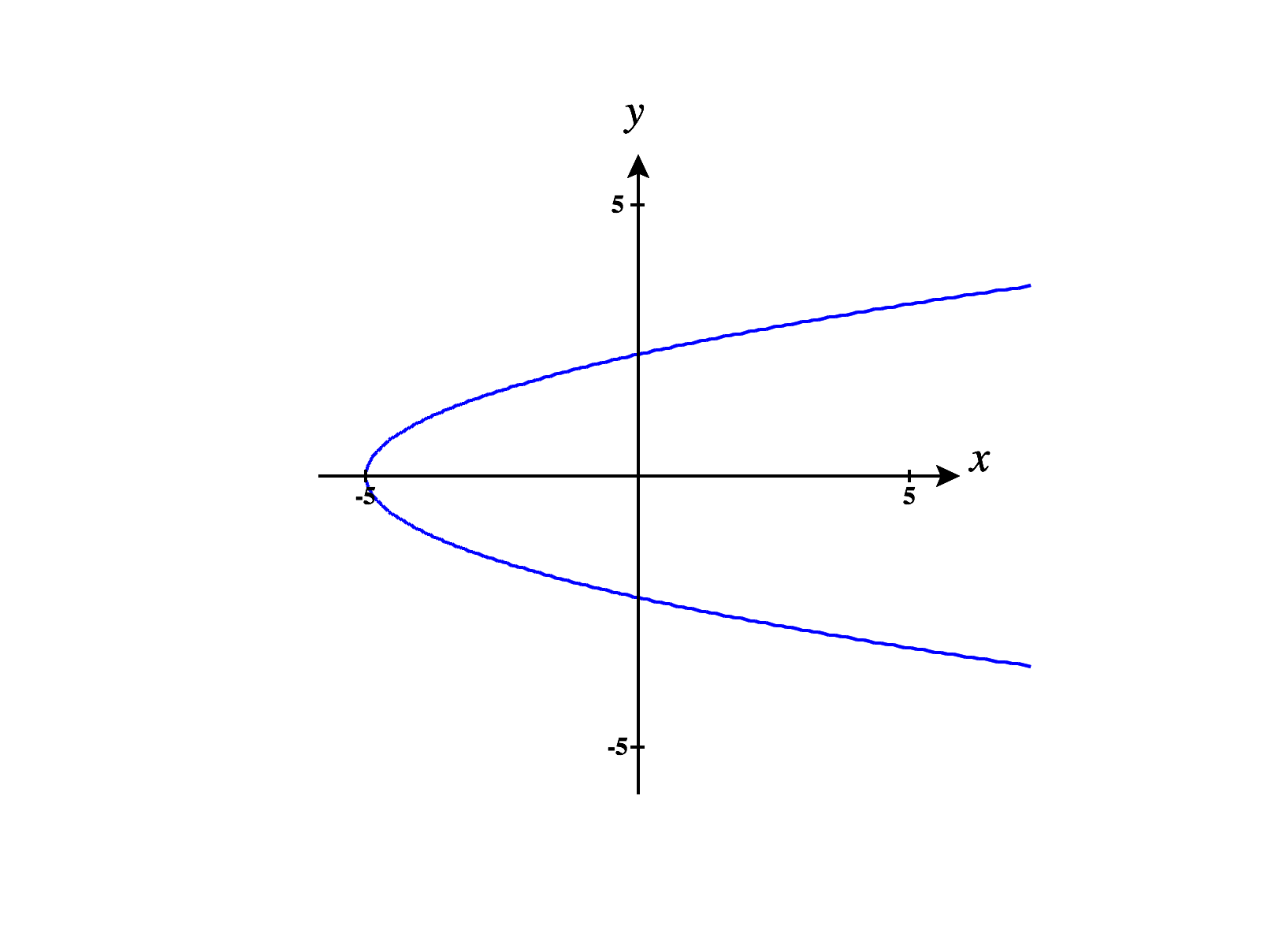
and the graph of $g(x,y) = C$ is a curve in $\mathbb {R}^2$ .

Now, suppose that the maximum value of $f(x,y)$ subject to the constraint $g(x,y)=C$ occurs at some point $(a,b)$ . Suppose we parametrize the curve $g(x,y)=C$ as $\vec {x}(t)$ , with $(a,b)=\vec {x}(t_0)$ . We can view $g(x,y)=C$ as a level curve of the function $g(x,y)$ , and then the gradient of $g(x,y)$ will always be perpendicular to the curve $g(x,y)=C$ .

More precisely, for any point $(x,y) = \vec {x}(t)$ on the curve $g(x,y)=C$ , we’ll have $\nabla g(x,y)$ is perpendicular to $\vec {x}'(t)$ . That is, $\nabla g(\vec {x}(t))\perp \vec {x}'(t)$ for all $t$ .

Next, let’s turn our attention back to $f$ . If $f$ has an absolute maximum subject to $g(x,y)=C$ , then $f(\vec {x}(t))$ has an absolute maximum at $t=t_0$ . This means that $f(\vec {x}(t))$ has a critical point at $t=t_0$ , so $\frac {d}{dt}f(\vec {x}(t))|_{t=t_0}=0$ . Using the chain rule, we can rewrite this as $\nabla f(\vec {x}(t_0))\cdot \vec {x}'(t)=0.$ So, both $\nabla f(a,b)$ and $\nabla g(a,b)$ are perpendicular to $\vec {x}'(t)$ . Since we are considering vectors in $\mathbb {R}^2$ , this means that $\nabla f(a,b)$ and $\nabla g(a,b)$ are parallel, so we can write $\nabla f(a,b) = \lambda \nabla g(a,b)$ for some constant $\lambda$ .

So, we can find candidate points for the absolute maximum (and similarly, the absolute minimum) of $f(x,y)$ subject to the constraint $g(x,y)=C$ by finding points where $\nabla f(a,b) = \lambda \nabla g(a,b).$ This observation generalizes to $\mathbb {R}^n$ .

Consider $\mathcal {C}^1$ functions $f,g:\mathbb {R}^n\rightarrow \mathbb {R}$ , and let $C$ be a constant. If $f$ has an absolute maximum or absolute minimum at $\vec {a}$ subject to the constraint $g(\vec {x}) = C$ , then there exists some scalar $\lambda$ such that $\nabla f(\vec {a}) = \lambda \nabla g(\vec {a}).$ The constant $\lambda$ is called a Lagrange Multiplier.

We can leverage this theorem into a method for finding absolute extrema of a function subject to a constraint, which we call the method of Lagrange multipliers.

To find the absolute extrema of a function $f(\vec {x})$ subject to a constraint $g(\vec {x})=C$ :

(a): Compute the gradients $\nabla f(\vec {x})$ and $\nabla g(\vec {x})$ .
(b): Solve the system of equations $\begin {cases} \nabla f(\vec {x}) = \lambda \nabla g(\vec {x})\\ g(\vec {x}) = C \end {cases}$ for $\vec {x}$ and $\lambda$ .
(c): The solutions to the system of equations in (2) are the critical points of $f(\vec {x})$ subject to $g(\vec {x}) = C$ . Classify these critical points in order to determine the absolute extrema.
If $g(\vec {x})=C$ is compact, we can determine the absolute extrema by comparing the values of $f$ at the critical points. In this case, absolute extrema are guaranteed to exist by the Extreme Value Theorem.

We’ll see how this process works in a couple of examples. First, we repeating an optimization problem which was previously done with substitution.

We’ll find the absolute maximum and absolute minimum of $f(x,y) = x^2-y^2$ subject to the constraint $x^2+y^2=1$ . Notice that $x^2+y^2=1$ is a compact region, so absolute extrema will exist.

If we let $g(x,y) = x^2+y^2$ , our constraint is $g(x,y) = 1$ .

Computing the gradients of $f$ and $g$ , we have

$\begin{align*} \nabla f(x,y) &= \answer{(2x, -2y)},\\ \nabla g(x,y) &= \answer{(2x, 2y)}. \end{align*}$

Setting up the system of equations $\begin {cases} \nabla f(\vec {x}) = \lambda \nabla g(\vec {x})\\ g(\vec {x}) = 1 \end {cases},$ we have

$\begin{align*} \nabla (2x,-2y) &= \lambda (2x, 2y)\\ x^2+y^2&=1\\ \end{align*}$

We can rewrite this as a system of three equations, $\begin {cases} 2x=2\lambda x\\ 2y=-2\lambda y\\ x^2 +y^2 =1 \end {cases}.$

From the first equation, we have either $x=0$ or $\lambda =1$ .

If $x=0$ , the third equation gives us $y=\pm 1$ . Thus, we obtain the critical points $(0,\pm 1)$ .

If $\lambda =1$ , the second equation gives us $y=0$ . Then, the third equation gives us $x = \pm 1$ . This gives us the critical points $(\pm 1, 0)$ .

Since we know that $f$ will have an absolute maximum and minimum subject to our constraint, we will compare the values at the critical points to determine the absolute maximum and minimum.

$\begin{align*} f(0,-1) &= -1\\ f(0,1) &= -1\\ f(-1,0) &= 1\\ f(1,0) &=1 \end{align*}$

We see that the absolute maximum of $f$ subject to our constraint is $1$ , and this occurs at the points $(\pm 1, 0)$ . The absolute minimum of $f$ subject to our constraint is $-1$ , and this occurs at the points $(0,\pm 1)$ .

Next, we’ll attempt to optimize $f(x,y) = 12-x^2-y^2$ subject to the constraint $y^2=x+5$ . Here, we’ll need to be a bit more careful, since the curve defined by $y^2=x+5$ is not compact, as it is unbounded.

However, Lagrange multipliers will still be helpful for finding critical points. We can rewrite our constaint as $y^2-x=5$ , and take $g(x,y) = y^2-x$ . So, we are optimizing $f(x,y)$ subject to the constraint $g(x,y) = 5$ .

We begin by finding the gradients of $f$ and $g$ .

$\begin{align*} \nabla f(x,y) &= \answer{(-2x, -2y)}\\ \nabla g(x,y) &= \answer{(-1, 2y)} \end{align*}$

Next, we solve the system $\begin {cases} \nabla f(\vec {x}) = \lambda \nabla g(\vec {x})\\ g(\vec {x}) = 5 \end {cases},$ which is $\begin {cases} (-2x,-2y) = \lambda (-1,2y)\\ y^2-x= 5 \end {cases}.$ We can rewrite this system as the three equations $\begin {cases} -2x = -\lambda \\ -2y = 2\lambda y\\ y^2-x= 5 \end {cases}.$ From the second equation, we have either $y=0$ , or $\lambda =-1$ .

If $y=0$ , the third equation gives us $x=-5$ . So, we have a critical point $(-5,0)$ .

If $\lambda =-1$ , the first equation gives us $x= -\frac {1}{2}$ . Then the third equation gives us $y=\pm \frac {3}{\sqrt {2}}$ . So, we have the critical points $\left (-\frac {1}{2}, \pm \frac {3}{\sqrt {2}}\right )$ .

In this case, we can’t determine the absolute maximum and absolute minimum by plugging in these points, since we aren’t optimizing over a compact region.

However, looking at the graph of $f$ over the curve $g(x,y) = 5$ , we can see that the absolute maximum occurs at the points $\left (-\frac {1}{2}, \pm \frac {3}{\sqrt {2}}\right )$ . Although there is a local minimum at $(-5,0)$ , this is not an absolute minimum, as there is no absolute minimum.