Parametric Curves

$\newenvironment {prompt}{}{} \newcommand {\DeclareMathOperator }[2]{\@OldDeclareMathOperator {##1}{##2}\immediate \write \myfile {\unexpanded {\DeclareMathOperator }{\unexpanded {##1}}{\unexpanded {##2}}}} \newcommand {\ungraded }[0]{} \newcommand {\reserved@a }[2]{} \newcommand {\HyperFirstAtBeginDocument }[0]{\AtBeginDocument } \newcommand {\reserved@a }[1]{} \newcommand {\reserved@a }[2]{} \newcommand {\vnameref }[1]{\unskip ~\nameref {##1}\@vpageref [\unskip ]{##1}} \newcommand {\ref }[0]{\@ifstar \@refstar \T@ref } \newcommand {\pageref }[0]{\@ifstar \@pagerefstar \T@pageref } \newcommand {\nameref }[0]{\@ifstar \@namerefstar \T@nameref } \newcommand {\reserved@a }[2]{} \newcommand {\reserved@a }[0]{\AtBeginDocument } \newcommand {\reserved@a }[1]{} \newcommand {\reserved@a }[2]{}$

We’ve dealt with several ways to describe curves in $\mathbb {R}^2$ :

As the graph of a function. For example, $f(x) = x^2$ .
As the set of points satisfying an equation. For example, the points $(x,y)$ such that $x^2 + y^2 = 1$ .
As the set of points satisfying an equation in another coordinate system. For example, $r = \sin (\theta )$ in polar coordinates.

Another way that we can describe a curve is using parametric equations. When describing a curve using parametric equations, we define $x$ and $y$ in terms of a third variable, often $t$ , called the parameter. We often think about $t$ as representing time, and imagine the curve being drawn out as $t$ increases. This gives us another way to describe curves in $\mathbb {R}^2$ , and potentially describe some new and strange curves.

We can describe the unit circle in $\mathbb {R}^2$ with the parametric equations

$\begin{align*} x & = \cos(t),\\ y & = \sin(t), \end{align*}$

for $0\leq t \leq 2\pi$ .

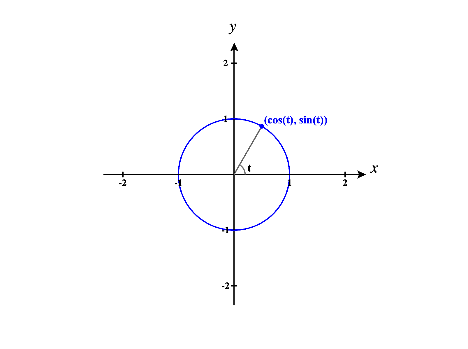
We can think of $t$ as giving the angle that a point makes with the positive axis. It can also be helpful to imagine $t$ as representing time, and the parametric equations tracing out the circle as time passes.

Consider the parametric equations for the unit circle in $\mathbb {R}^2$ :

$\begin{align*} x & = \cos(t),\\ y & = \sin(t), \end{align*}$

for $0\leq t \leq 2\pi$ .

We can combine these equations into a single vector, $\vec {x}(t) = (\cos (t), \sin (t))\textrm { for }0\leq t\leq 2\pi .$

We can visualize the vectors $\vec {x}(t)$ tracing out the unit circle as $t$ goes from $0$ to $2\pi$ .

Notice that we are blurring the distinction between vectors and points. Although we can think of $vec{x}(t)$ as a position vector, we would more commonly think of $\vec {x}(t)$ as a point on a curve. Although this might seem a bit sloppy, it will prove very useful throughout the course. Although intuitively we might prefer to use points, a lot of the computations tools that we’ll require are more appropriately used with vectors.

We have defined a function $\vec {x}$ from the interval $[0,2\pi ]\subset \mathbb {R}$ to $\mathbb {R}^2$ , and this idea provides the motivation behind our definition for paths.

Parametric Curves in $\mathbb {R}^n$

A path in $\mathbb {R}^n$ is a continuous function $\vec {x}:I\subset \mathbb {R}\rightarrow \mathbb {R}^n,$ where $I\subset \mathbb {R}$ is an interval.

This is also called a parametrized curve or parametric curve. When we wish to emphasize that $\vec {x}(t)$ is a vector, we’ll call it the position vector.

We’ll focus on the cases $n=2$ and $n=3$ in this course.

We defined a path as a continuous function, however, we haven’t said what it means for a multivariable function to be continuous. We’ll come back to this later, and we’ll give a rigorous definition for continuity. For now, this should fit with your intuition: you can draw the path without lifting your pencil from the paper.

Sometimes we care more about the image of a path than how the path is drawn out, and then we refer to a curve.

A curve $C$ in $\mathbb {R}^n$ is the image of some path $\vec {x}:I\subset \mathbb {R}\rightarrow \mathbb {R}^n$ .

In this case, we say that $\vec {x}$ is a parametrization for the curve $C$ .

The difference between a curve and a path is largely a matter of perspective: when working with a curve, we pay attention to what is drawn; when working with a path, we care about how it is drawn.

There are many different parametrizations for a given curve.

Consider again the unit circle $C$ in $\mathbb {R}^2$ . Which of the following are parametrizations for $C$ ?

$\vec {x}(t) = (\cos (t),\sin (t))$ for $0\leq t\leq 2\pi$ $\vec {x}(t) = (\sin (t),\cos (t))$ for $0\leq t\leq \pi$ $\vec {x}(t) = (t, \pm \sqrt {1-t^2})$ for $-1\leq t\leq 1$ $\vec {x}(t) = (\sin (2\pi t),\cos (2\pi t))$ for $0\leq t\leq 1$ $\vec {x}(t) = (\cos (t),\sin (t))$ for $-10\leq t\leq 10$

In this example, we review a parametrization for the line through points $\vec {a}$ and $\vec {b}$ in $\mathbb {R}^n$ .

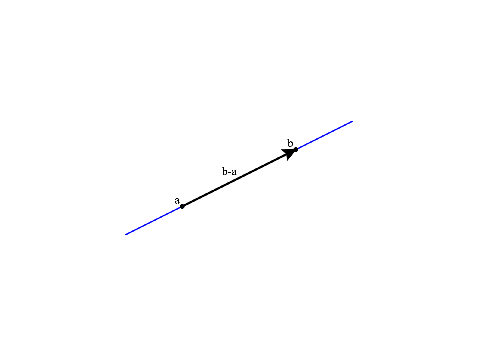
Given points $\vec {a}$ and $\vec {b}$ in $\mathbb {R}^n$ , we obtain a vector starting at $\vec {a}$ and ending at $\vec {b}$ by taking $\vec {b}-\vec {a}$ . This vector is parallel to the line through $\vec {a}$ and $\vec {b}$ . Then, taking scalar multiples $t(\vec {b} - \vec {a})$ for $t\in \mathbb {R}$ , we have a line parallel to the line through $\vec {a}$ and $\vec {b}$ . Finally, we add one of the points, $\vec {a}$ , to ensure that our line passes through these two points. Thus, we arrive at our parametrization, $\vec {l}(t) = \vec {a} + t(\vec {b}-\vec {a})\textrm { for }t\in \mathbb {R}.$

In this example, we see how we can obtain new transformations from old ones, using linear algebra and simple transformations.

Recall the parametrization for the unit circle in $\mathbb {R}^2$ , $\vec {x}(t) = (\cos (t), \sin (t))\textrm { for }0\leq t\leq 2\pi .$

Now, consider the ellipse below.

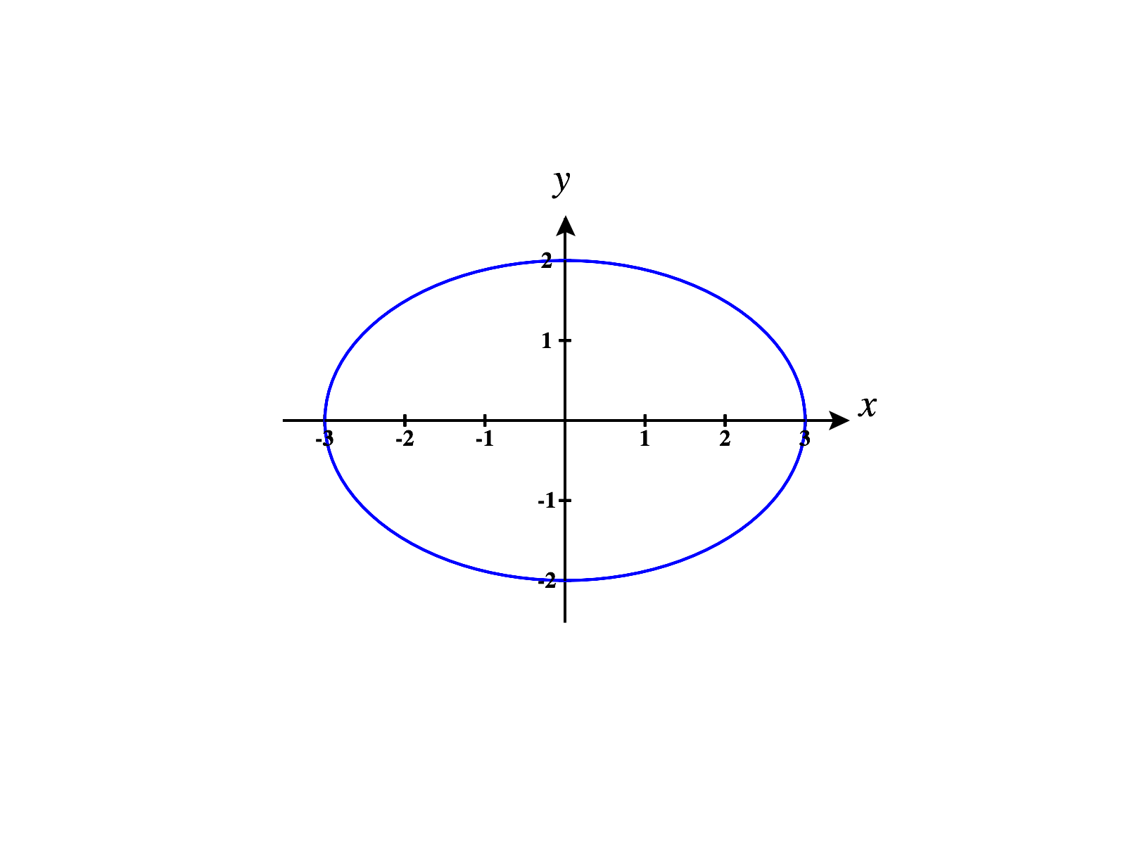
We can think of this ellipse as the result of stretching the unit circle horizontally by a factor of $3$ and vertically by a factor of $2$ . That is, we are applying the linear transformation $\left (\begin {array}{cc} 3 & 0\\ 0 & 2 \end {array}\right ).$ We can apply this to the parametrization for the unit circle, in order to parametrization for the ellipse.

$\begin{align*} \vec(y)(t) &= \left(\begin{array}{cc} 3 & 0\\ 0 & 2 \end{array}\right)\left(\begin{array}{c}\cos(t)\\\sin(t)\end{array}\right),\\ &= (3\cos(t), 2\sin(t)). \end{align*}$

Thus, we have a parametrization for the ellipse given by $\vec {y}(t) = (3\cos (t), 2\sin (t))\textrm { for }0\leq t\leq 2\pi .$

Next, consider the following ellipse.

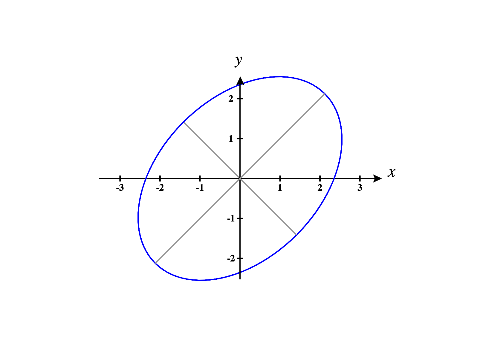
We can obtain this from our previous ellipse by counterclockwise rotation of $\pi /4$ . The matrix for this linear transformation is $\left (\begin {array}{cc} \cos (\pi /4) & -\sin (\pi /4)\\ \sin (\pi /4) & \cos (\pi /4) \end {array}\right ) = \left (\begin {array}{cc} \answer {1/\sqrt {2}} & \answer {-1/\sqrt {2}}\\ \answer {1/\sqrt {2}} & \answer {1/\sqrt {2}} \end {array}\right ).$ Applying this rotation to our parametrization for the previous ellipse, we obtain a parametrization for our new ellipse. $\vec {z}(t) = \answer {(3/\sqrt {2}\cos (t) -2/\sqrt {2}\sin (t), 3/\sqrt {2}\cos (t) + 2/\sqrt {2}\sin (t))}\textrm { for }0\leq t\leq 2\pi$

Finally, we consider an ellipse in $\mathbb {R}^3$ , shown below.

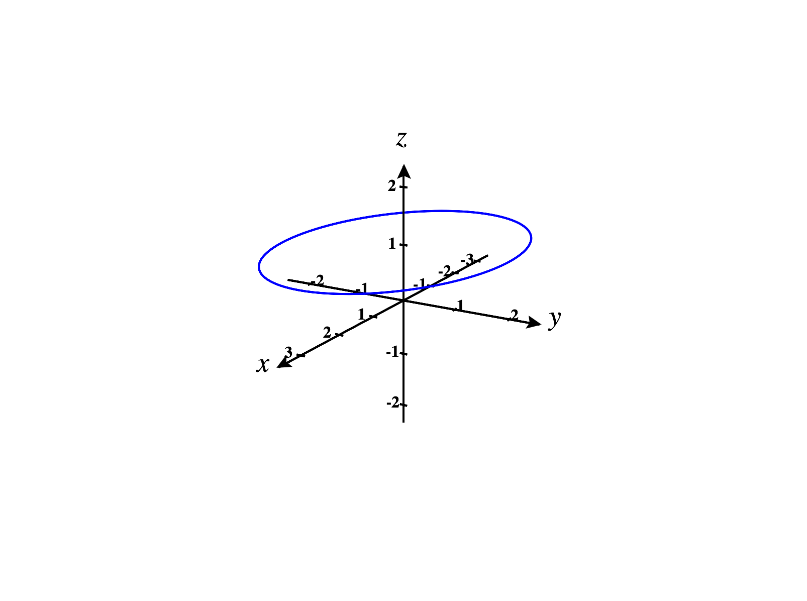
This ellipse is parallel to the $xy$ -plane, and will have constant $z$ -coordinate of $1$ . Note the similarity to the first ellipse we considered. A parametrization for this ellipse can be obtained by taking the parametrization $\vec {y}$ for our first ellipse in $\mathbb {R}^2$ , and appending the constant $z$ -coordinate. $\vec {a}(t) = \answer {(3\cos (t), 2\sin (t),1)}\textrm { for }0\leq t\leq 2\pi$

Examples in $\mathbb {R}^3$

In this section, we give examples of parametrizations of a couple of more complicated curves in $\mathbb {R}^3$ , taking advantage of our previous experience with cylindrical coordinates.

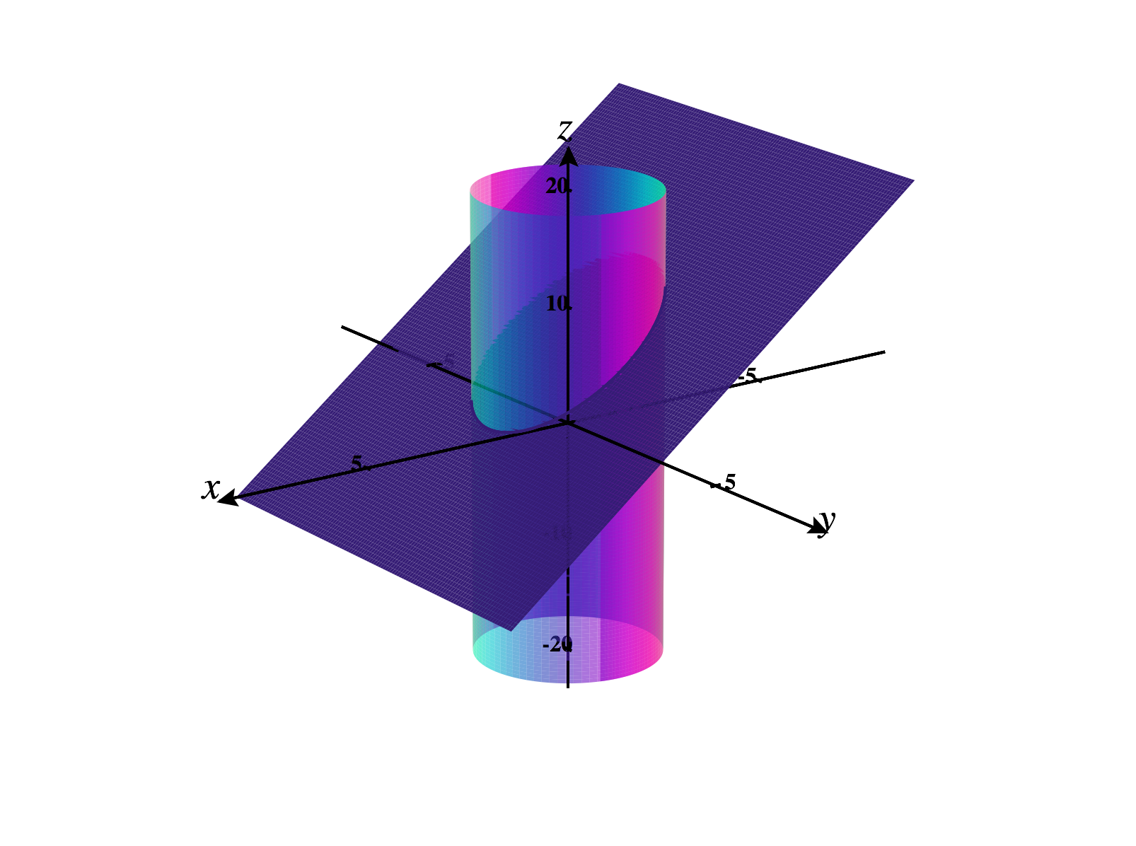
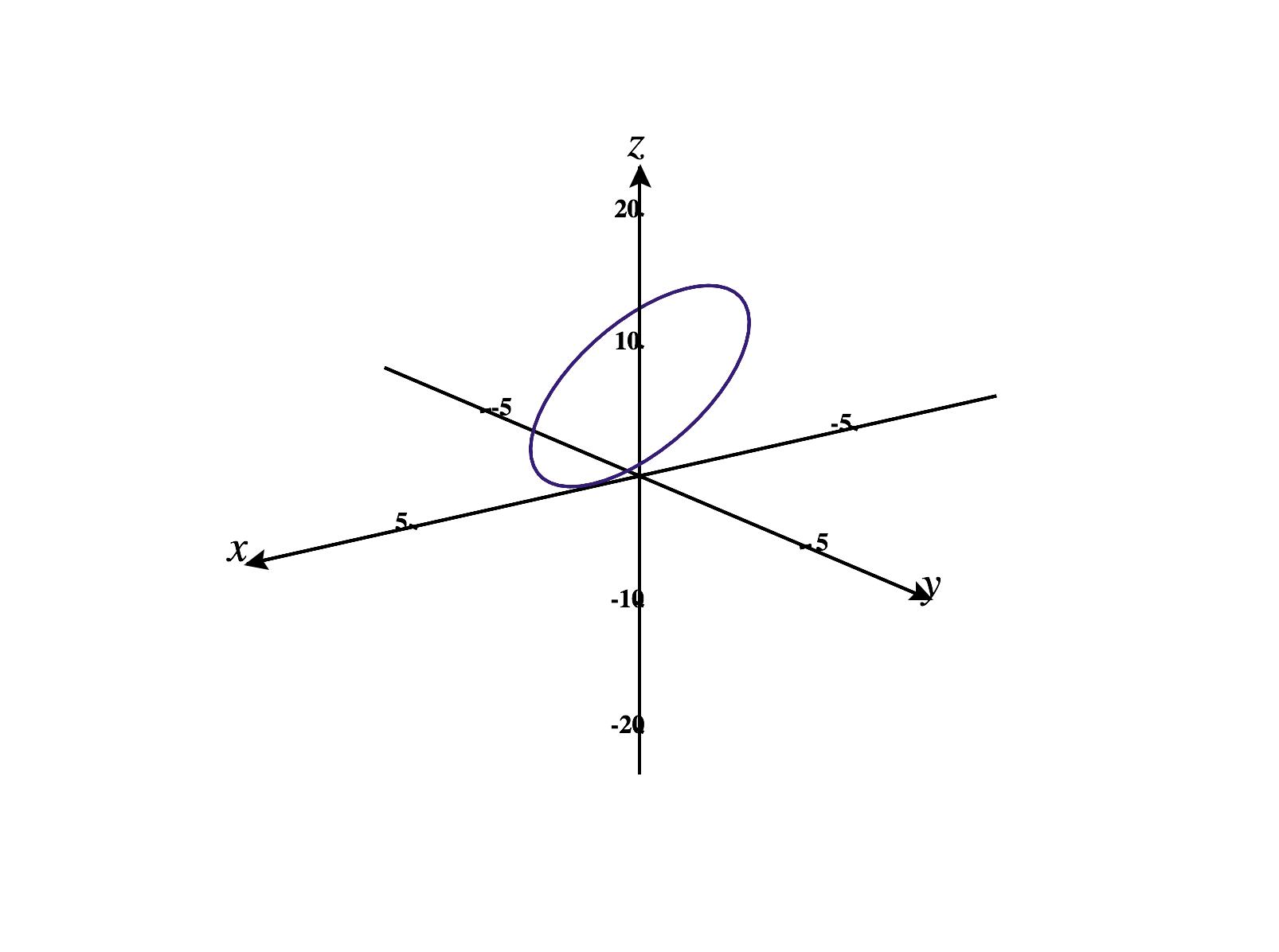
We’ll parametrize the intersection of the cylinder $x^2 + y^2 = 4$ and the plane $z = 7-3x$ in $\mathbb {R}^3$ , pictured below.

Our $x$ and $y$ coordinates must satisfy $x^2 + y^2 = 4$ , which would define a circle, if we were in $\mathbb {R}^2$ . Recalling our parametrizations for circles, these coordinates can be written as

$\begin{align*} x(t) &= 2\cos(t)\\ y(t) &= 2\sin(t) \end{align*}$

for $0\leq t\leq 2\pi$ .

It remains to write the $z$ -coordinate in terms of the parameter $t$ . Turning our attention to the equation for the plane, $z = 7-3x$ , we have $z$ expressed in terms of $x$ . Since we have expressed $x$ in terms of $t$ , we can make this substitution to describe $z$ in terms of $t$ , $z(t) = \answer {7-6\cos (t)}.$

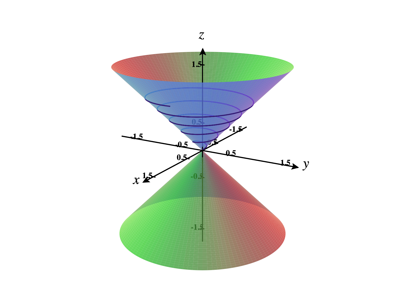
Putting all of this together, we have a parametrization for this intersection given by $\vec {x}(t) = \answer {(2\cos (t),2\sin (t),7-6\cos (t))} \textrm { for } 0\leq t\leq 2\pi .$

Consider the curve below, which lies on the cone $z^2 = x^2 + y^2$ , and makes five rotations around the $z$ -axis as the height ranges from $0$ to $1$ . We’ll refer to this curve as a “tornado.”

We’ll parametrize this curve by thinking about it in cylindrical coordinates, using the height as the parameter.

First, let’s consider what’s happening with the $z$ -coordinate. Since the height of the tornado rangers from $0$ to $1$ , so will $z$ . We’ll set $z = t$ , with $0\leq t\leq 1$ , and express $x$ and $y$ in terms of $t$ as well.

Now, we turn our attention to the angle $\theta$ . As the height ranges from $0$ to $1$ , the tornado makes five revolutions, so $\theta$ should range from $0$ to $10\pi$ . Thus, expressing $\theta$ in terms of $t$ , we let $\theta = 10\pi t$ .

Next, we consider the radius $r$ . Since we are on the cone $z^2 = x^2 + y^2$ , we have $z^2 = r^2$ . Since $z\geq 0$ , we have $z = r$ . Thus, we can write $r$ in terms of $t$ as $r = t$ .

Finally, putting all of this together with $x = r\cos \theta$ and $y = r\sin \theta$ , we have a parametrization for the tornado given by $\vec {x}(t) = \answer {(t\cos (10\pi t), t\sin (10\pi t), t)} \textrm { for } t\in [0,1].$

Images were generated using CalcPlot3D.

Parametric Curves in \mathbb {R}^n

Examples in \mathbb {R}^3

Parametric Curves in $\mathbb {R}^n$

Examples in $\mathbb {R}^3$