You are about to erase your work on this activity. Are you sure you want to do this?
Updated Version Available
There is an updated version of this activity. If you update to the most recent version of this activity, then your current progress on this activity will be erased. Regardless, your record of completion will remain. How would you like to proceed?
Mathematical Expression Editor
We introduce the idea of a vector at every point in space.
1 Types of functions
When we started on our journey exploring calculus, we investigated functions \(f:\R \to \R \).
Typically, we interpret these functions as being curves in the \((x,y)\)-plane:
We’ve also studied
vector-valued functions \(\vec {f}:\R \to \R ^n\). We can interpret these functions as parametric curves
in space:
We’ve also studied functions of several variables \(F:\R ^n \to \R \). We can interpret
these functions as surfaces in \(\R ^{n+1}\). For example if \(n=2\), then \(F:\R ^2\to \R \) plots a surface in \(\R ^3\):
Now we are ready for a new type of function.
2 Vector fields
Now we will study vector-valued functions of several variables:
\[ \vec {F}:\R ^n\to \R ^n \]
We interpret these
functions as vector fields, meaning for each point in the \((x,y)\)-plane we have a vector.
To some extent functions like this have been around us for a while, for if
\[ G:\R ^n\to \R \]
then \(\grad G\) is a
vector-field. Let’s be explicit and write a definition.
A vector field in \(\R ^n\) is a
function
\[ \vec {F}: \R ^n\to \R ^n \]
where for every point in the domain, we assign a vector to the range.
Consider the following table describing a vector field \(\vec {F}\):
Note that with the first choice, the lengths of the
vectors is changing, and that does not appear to be the case with our vector
field.
The second choice is not a vector field.
The third choice is not a vector field.
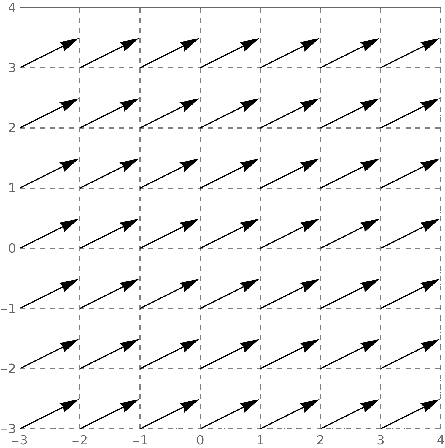
The fourth choice is a constant vector field, and is the correct answer.
3 Properties of vector fields
As we will see in the chapters to come, there are two important qualities of vector
fields that we are usually on the look-out for. The first is rotation and the second is
expansion. In the sections to come, we will make precise what we mean by rotation
and expansion. In this section we simply seek to make you aware that these are the
fundamental properties of vector fields.
3.1 Radial fields
Very loosely speaking a radial field is one where the vectors are all pointing toward a
spot, or away from a spot. Let’s see some examples of radial vector fields.
Here
we see \(\vec {F}(x,y) = \vector {\frac {x}{\sqrt {x^2+y^2}},\frac {y}{\sqrt {x^2+y^2}}}\).
Those vectors are all pointing away from the central point!
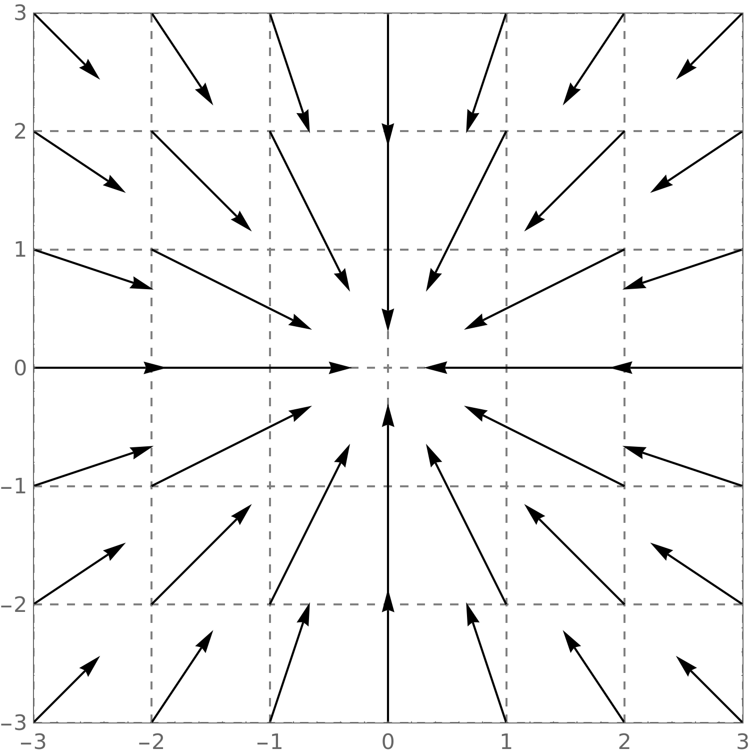
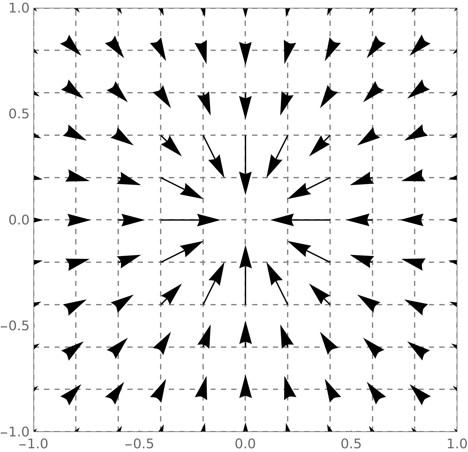
Here we see \(\vec {G}(x,y) = \vector {\frac {-x}{x^2+y^2},\frac {-y}{x^2+y^2}}\).
Those vectors are all pointing toward the central point.
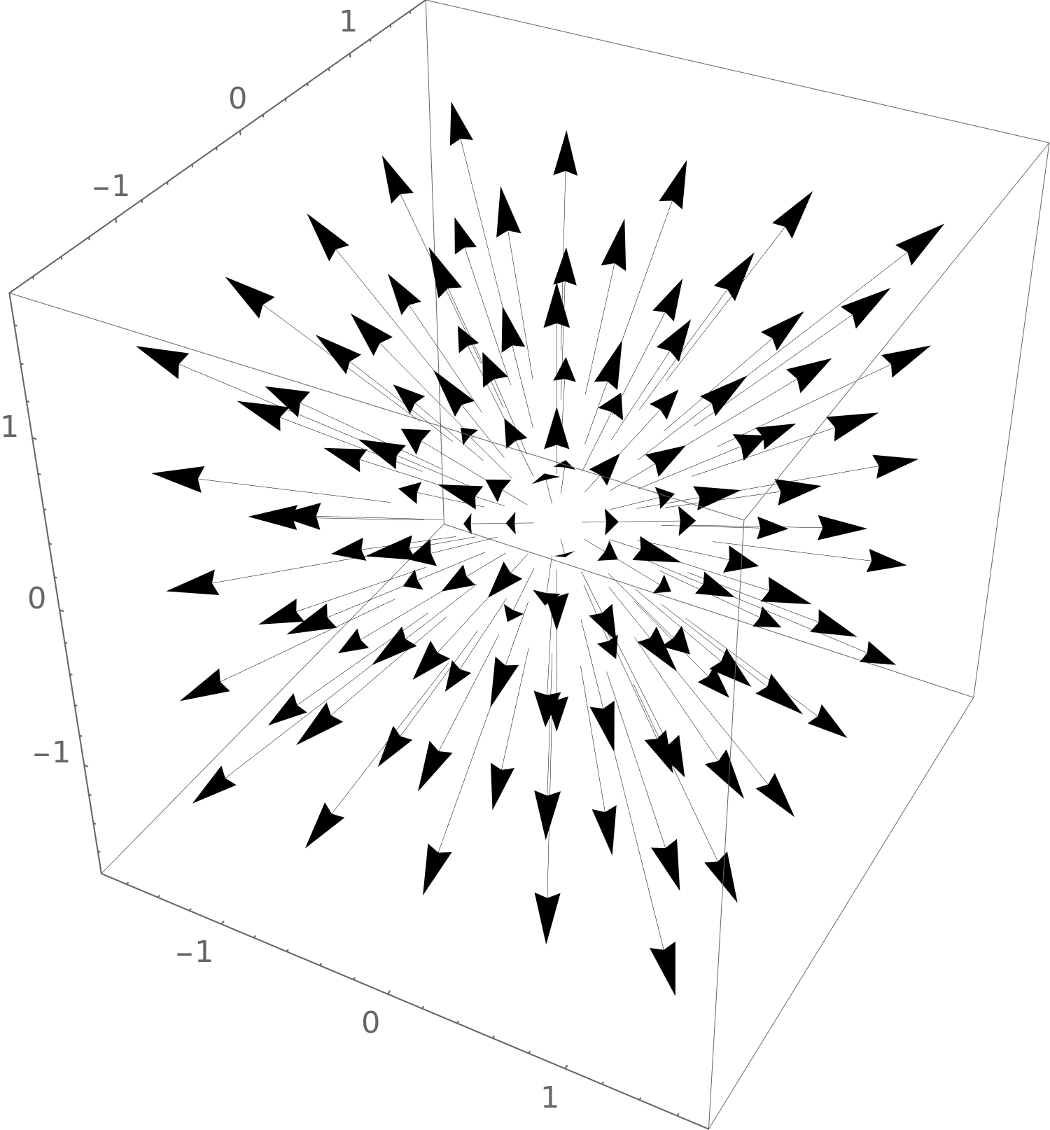
Here we see \(\vec {H}(x,y,z) = \vector {x,y,z}\).
This is a three-dimensional vector field where all the vectors are
pointing away from the central point.
Each of the vector fields above is a radial vector field. Let’s give an explicit
definition.
A radial vector field is a field of the form \(\vec {F}:\R ^n\to \R ^n\) where
Some fields look like they are expanding and are. Other fields look like the are
expanding but they aren’t. In the sections to come, we’re going to use calculus to
precisely define what we mean by a field “expanding.” This property will be called
divergence.
3.2 Rotational fields
Vector fields can easily exhibit what looks like “rotation” to the human eye. Let’s
show you a few examples.
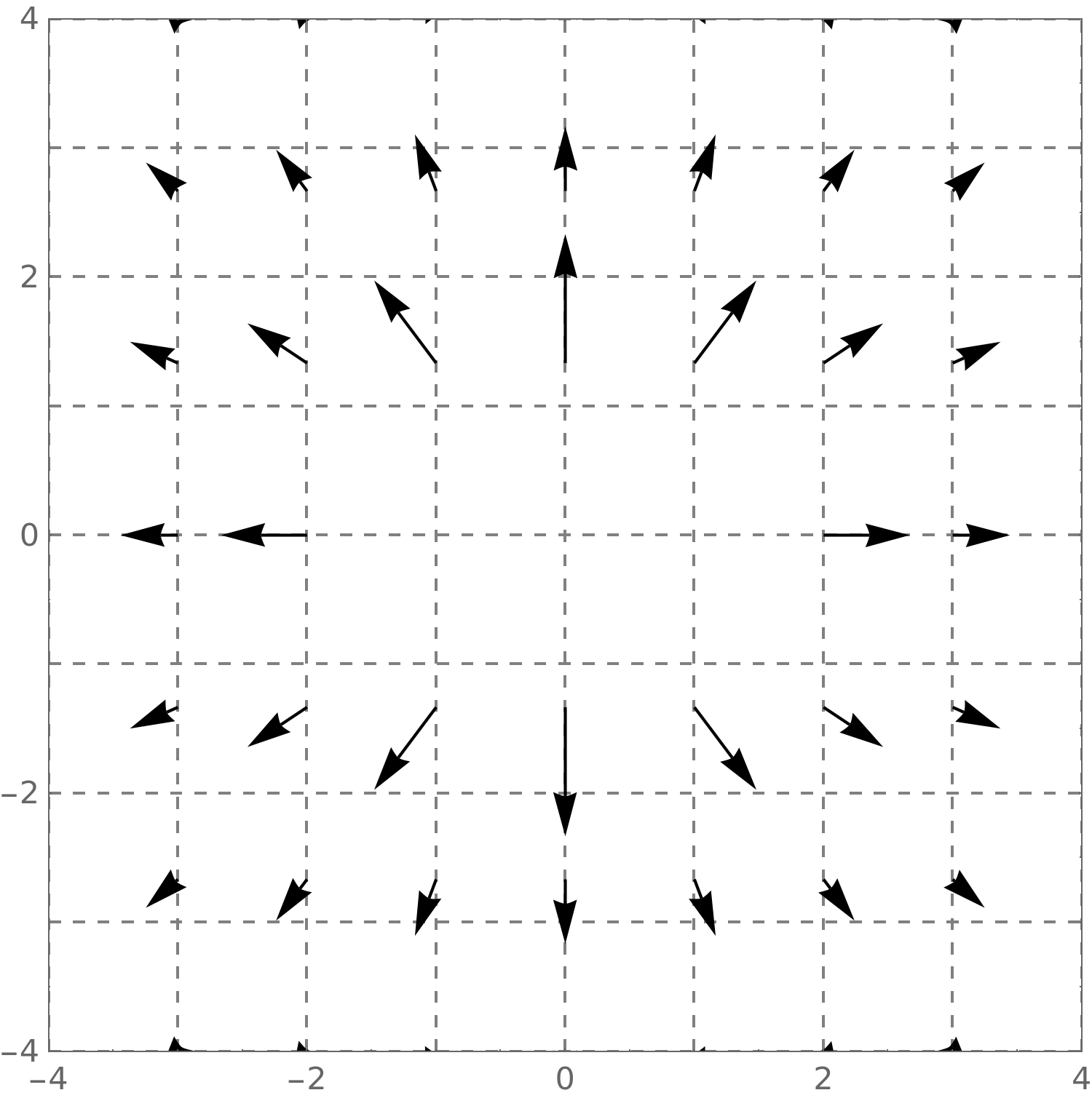
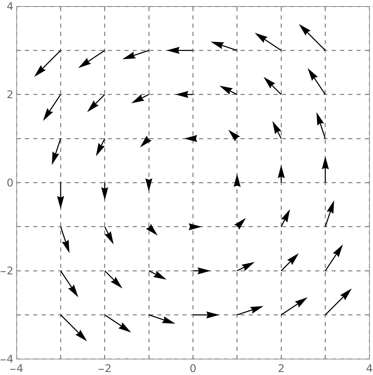
Here we see \(\vec {F}(x,y) = \vector {-y,x}\).
This vector field looks like it has
counterclockwise rotation.
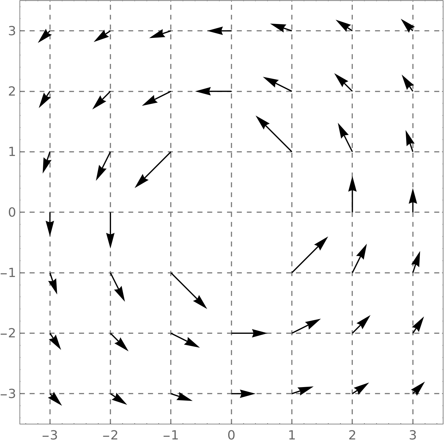
This vector field looks like it has clockwise rotation.
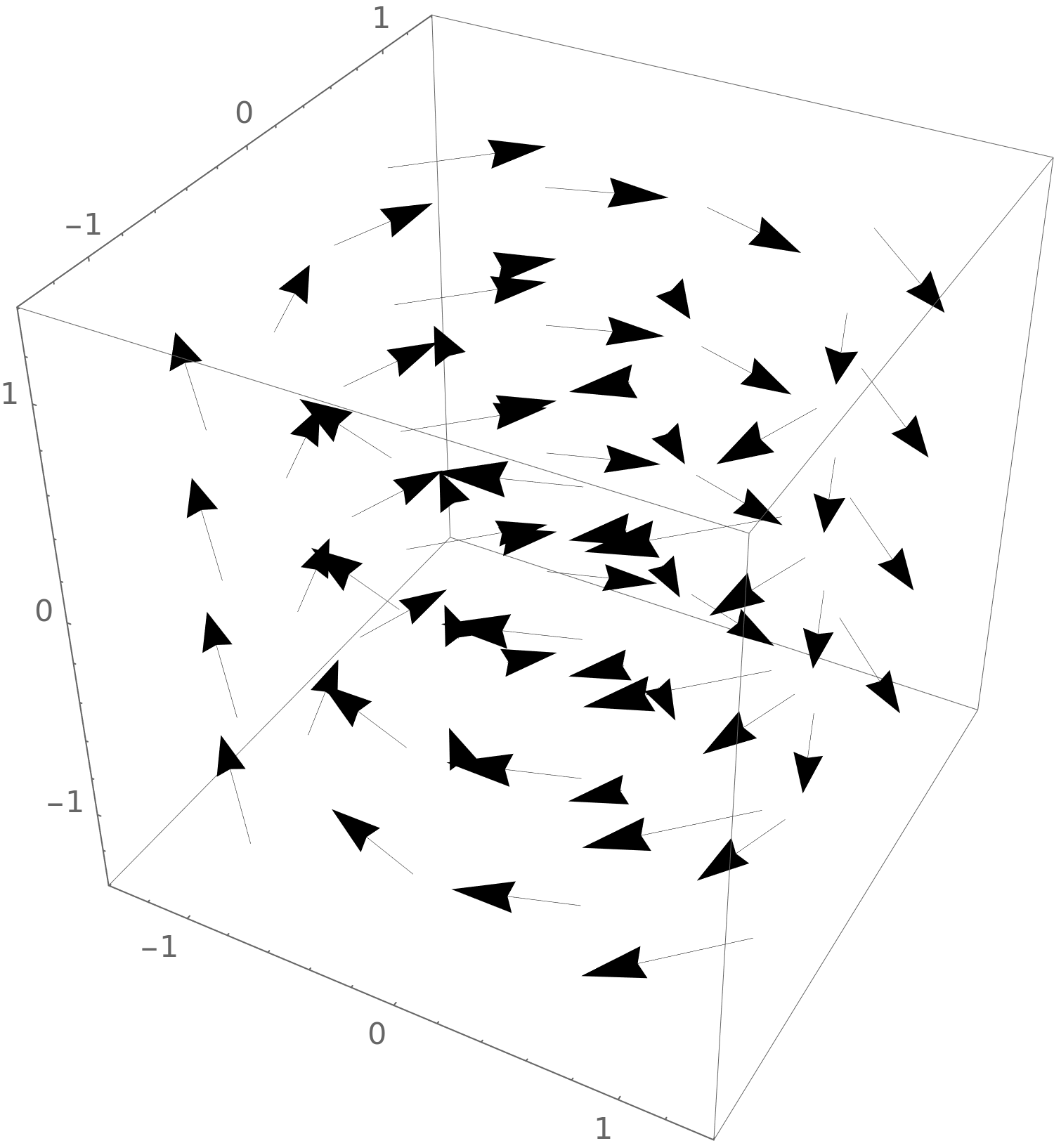
At this point, we’re going to give some “spoilers.” It turns out that from a local
perspective, meaning looking at points very very close to each other, only the first
example exhibits “rotation.” While the second example looks like it is “rotating,” as
we will see, it does not exhibit “local rotation.” Moreover, in future sections we will
see that rotation (even local rotation) in three-dimensional space must always happen
around some “axis” like this:
In the sections to come, we will use calculus to
precisely explain what we mean by “local rotation.” This property will be called
curl.
4 Gradient fields
In this final section, we will talk about fields that arise as the gradient of some
differentiable function. As we will see in future sections, these are some of the nicest
vector fields to work with mathematically.
Consider any differentiable function \(F:\R ^n\to \R \). A gradient field is a vector field \(\vec {G}:\R ^n\to \R ^n\) where
\[ \vec {G} = \grad F. \]
Note,
since we are assuming \(F\) is differentiable, we are also assuming that \(\vec {G}\) is defined for all
points in \(\R ^n\).
Let’s take a look at a gradient field.
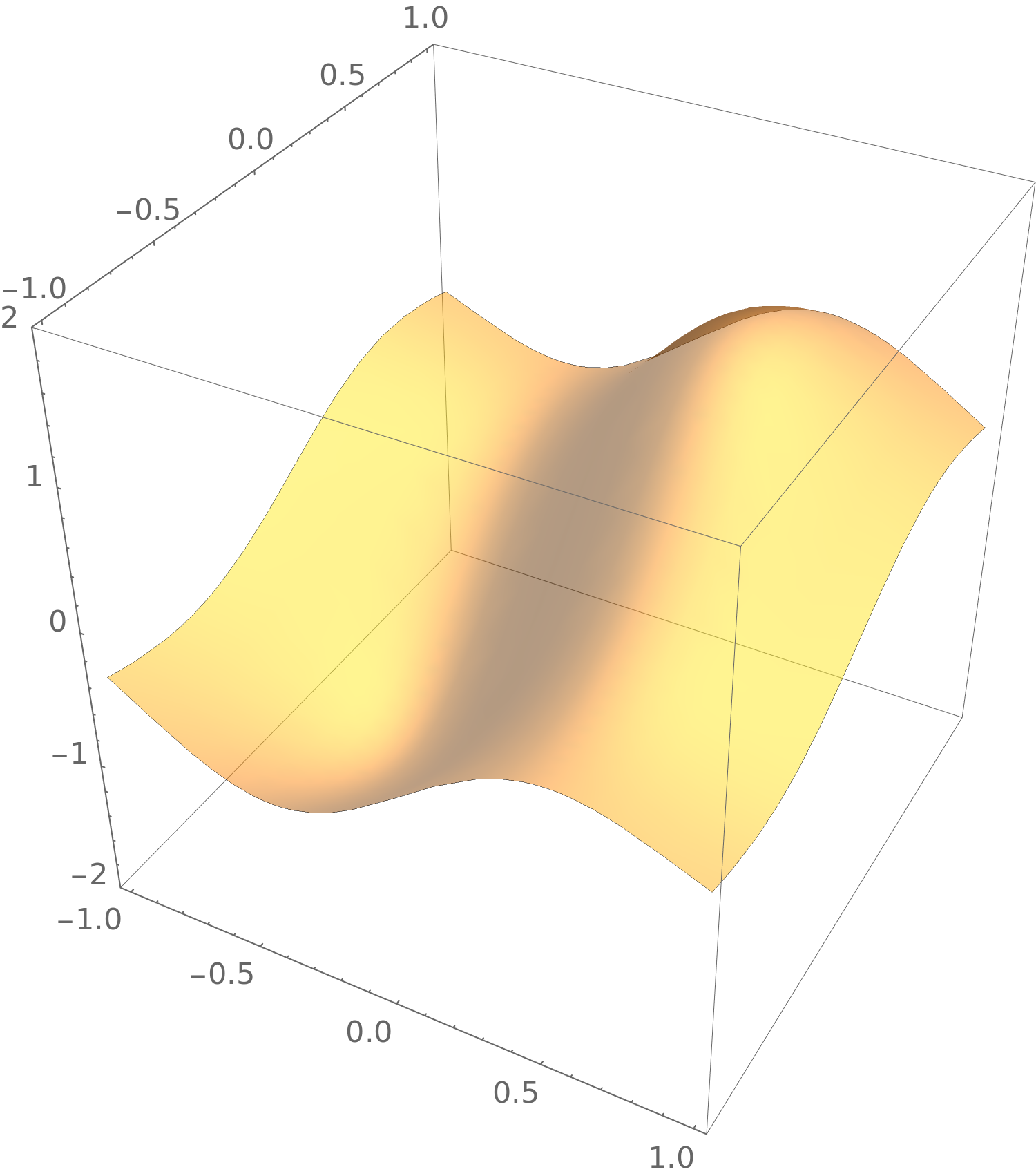
Consider \(F(x,y) = \frac {\sin (3x)+\sin (2y)}{1+x^2+y^2}\). A plot of this function looks like this:
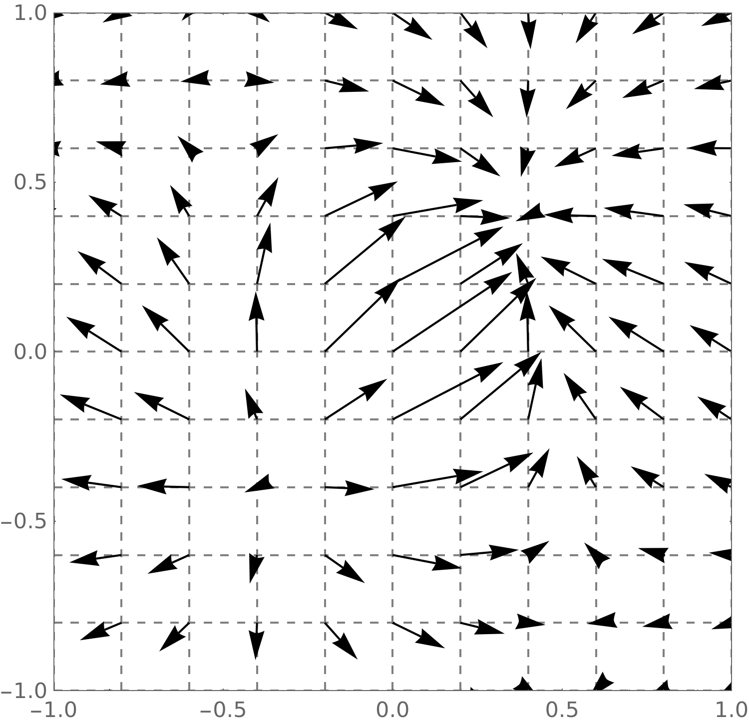
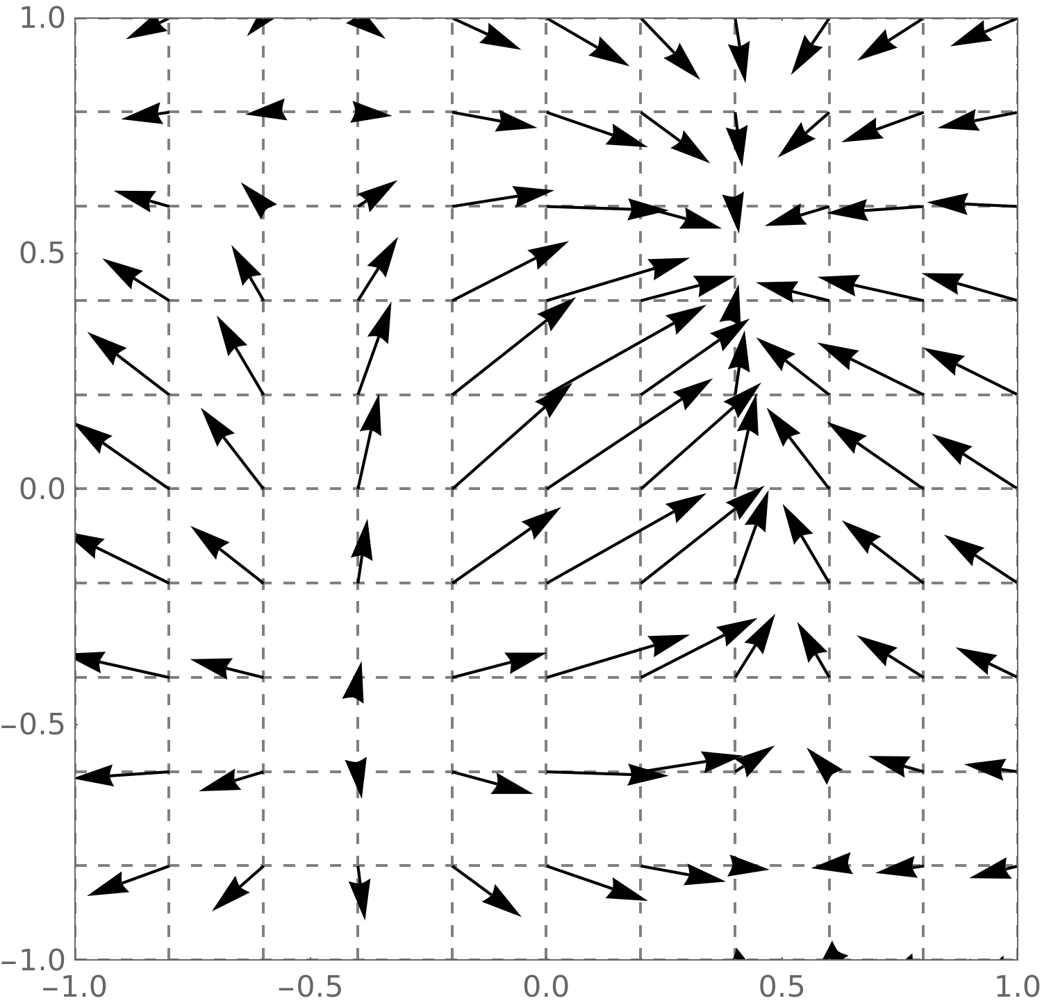
The gradient field of \(F\) looks like
this:
Note we can see the vector pointing in the initial direction of greatest
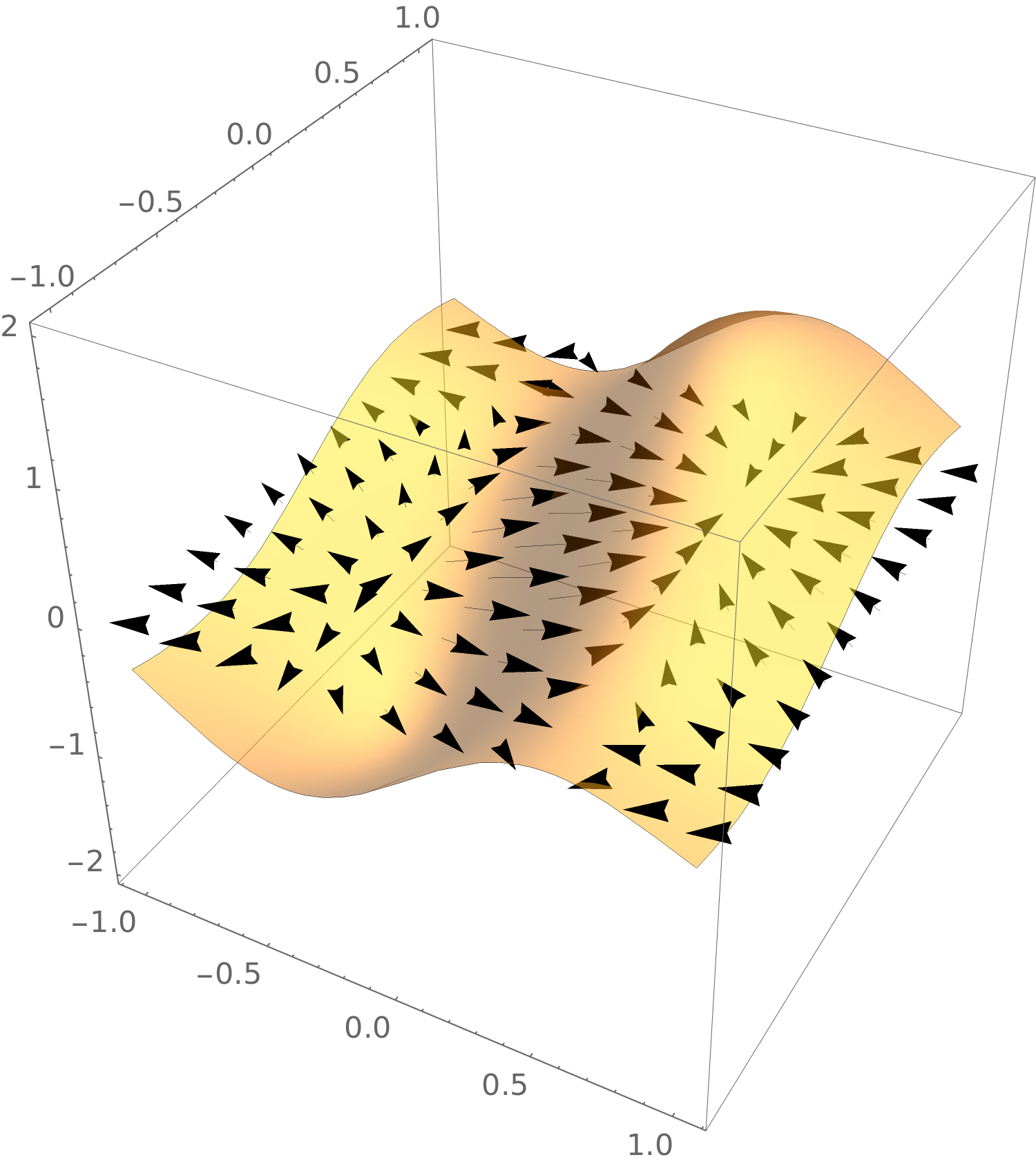
increase. Let’s see a plot of both together:
Remind me, what direction do gradient vectors point?
Gradient vectors point to
the maximum. Gradient vectors point up. Gradient vectors point in the initial
direction of greatest increase.
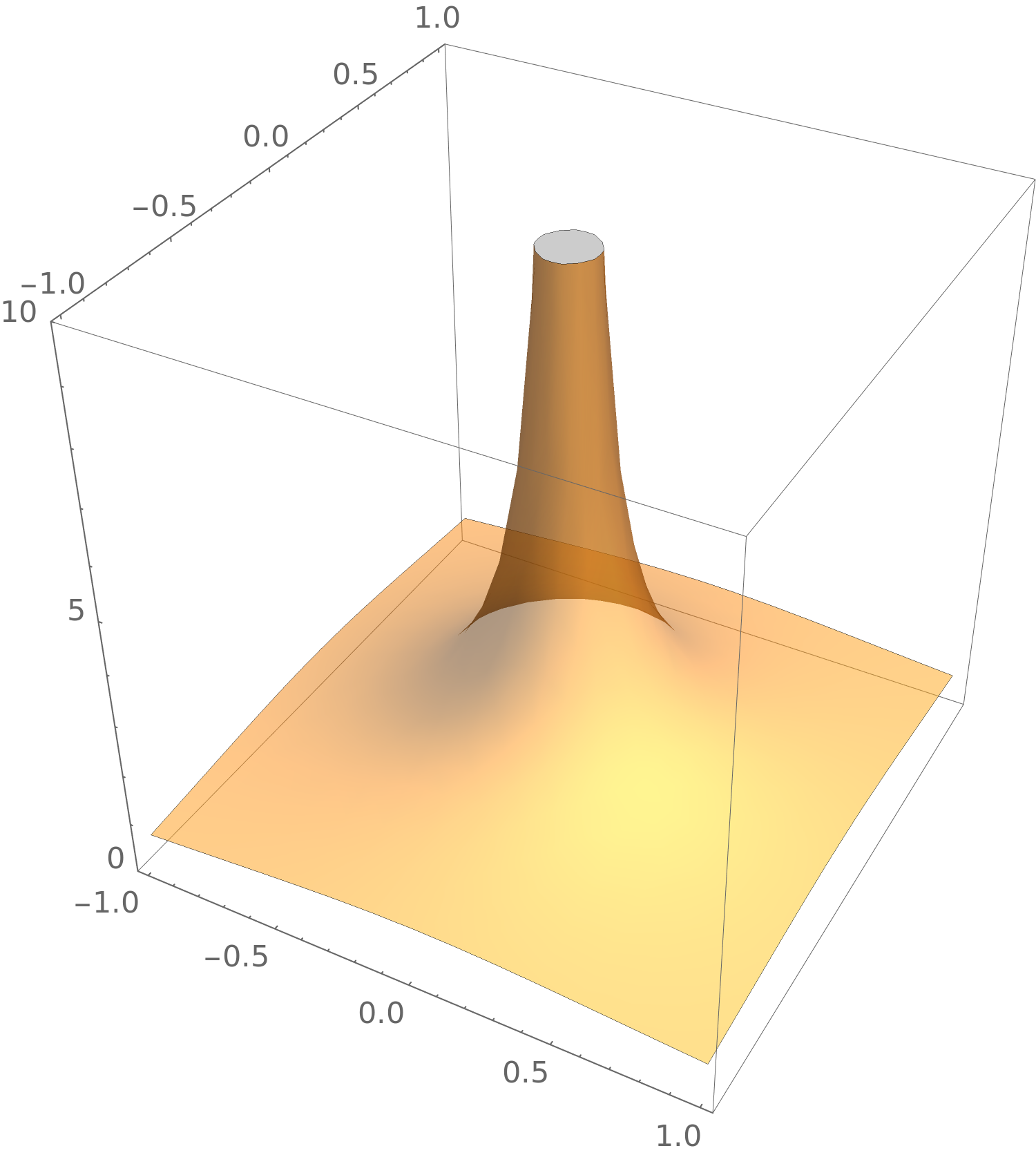
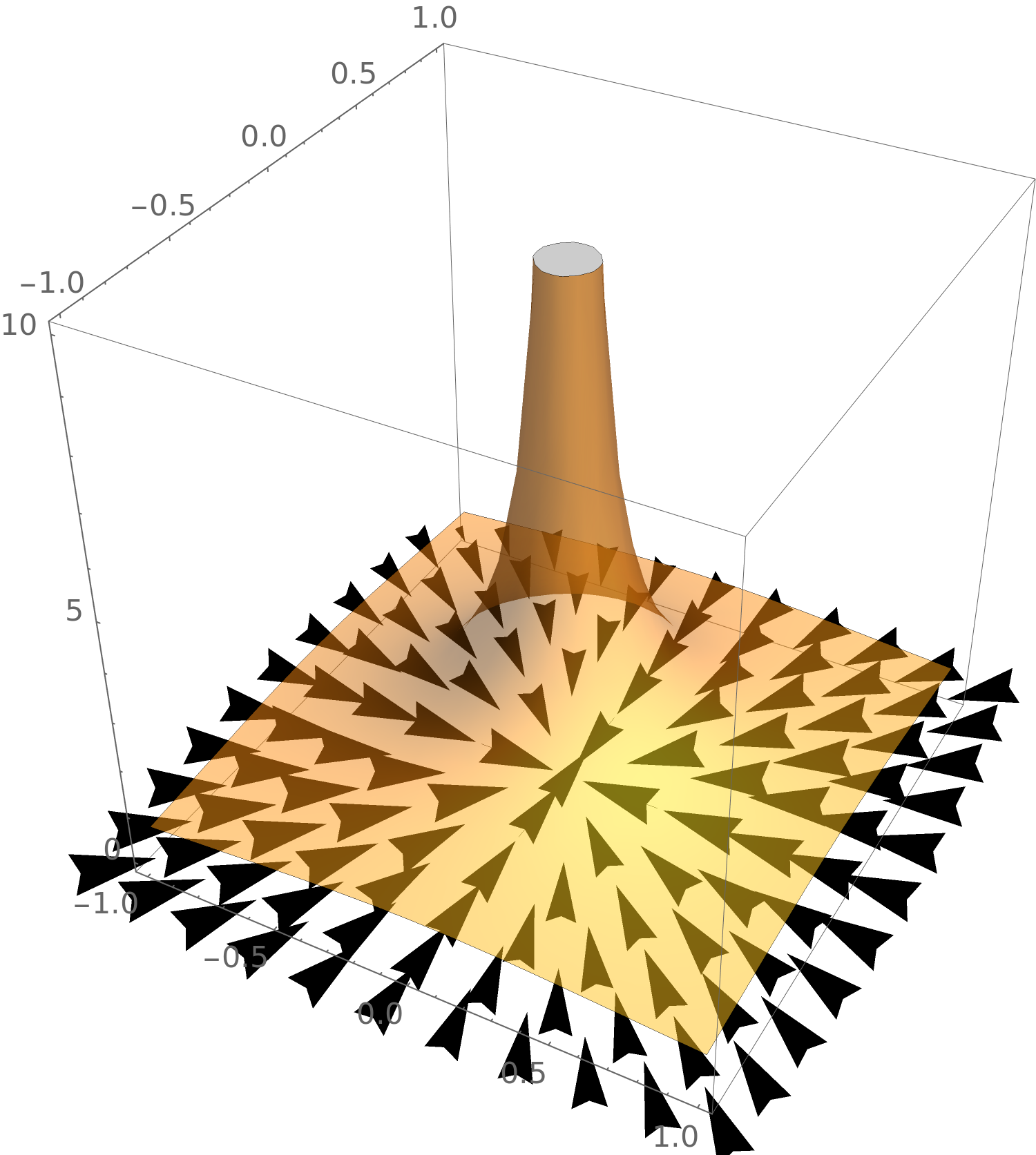
Now consider \(F(x,y) = \frac {1}{\sqrt {x^2+y^2}}\). A plot of this function looks like this:
Note we can see the vector pointing in the
initial direction of greatest increase. Let’s see a plot of both together:
5 The shape of things to come
Now we present the beginning of a big idea. By the end of this course, we hope to
give you a glimpse of “what’s out there.” For this we’re going to need some notation.
Think of \(A\) and \(B\) as sets of numbers, like \(A=\R \) or \(A=\R ^n\) or \(B=\R \) or \(B=\R ^n\).
\(C(A,B)\) is the set of continuous functions from \(A\) to \(B\).
\(C^1(A,B)\) is the set of differentiable functions from \(A\) to \(B\) whose first-derivative is
continuous.
\(C^2(A,B)\) is the set of differentiable functions from \(A\) to \(B\) whose first and second
derivatives are continuous.
\(C^n(A,B)\) is the set of differentiable function from \(A\) to \(B\) where the first \(n\)th derivatives
are continuous.
\(C^\infty (A,B)\) is the set of differentiable functions from \(A\) to \(B\) where all of the derivatives
are continuous.
Here is a deep idea:
The gradient turns functions of several variables into vector
fields.
Now we give a method to determine if a field is a gradient field.
Clairaut A vector field \(\vec {G}(x,y) = \vector {M(x,y),N(x,y)}\), where \(M\) and \(N\) have continuous partial derivatives, is a gradient
field if and only if
\[ \pp [N]{x} -\pp [M]{y} = 0 \]
for all \(x\) and \(y\).
Let’s take a second and think about the gradient as a
function on functions. Let \(C^\infty (A,B)\) be the set of all function from \(A\) to \(B\) whose \(i\)th-derivatives
are continuous for all values of \(i\). The gradient takes functions of several variables and
maps them to vector fields:
So \(\vec {G}(x,y) = \vector {M(x,y),N(x,y)}\) if and only if there is some function \(F:\R ^2\to \R \) where
\[ \pp [F]{x} = M \quad \text {and}\quad \pp [F]{y} = N \]
but if all the partial derivatives are
continuous, then:
And so we see \(\pp [N]{x} -\pp [M]{y} = 0\), and thus \(\vec {G}\) is a gradient field. Now let’s try to find a potential function.
To do this, we’ll antidifferentiate—in essence we want to “undo” the gradient. Write
with me:
\begin{align*} \int M(x,y) \d x &= \int \left (\answer [given]{2x+3y}\right ) \d x \\ &= \answer [given]{x^2+3xy} + c(y) \end{align*}
where \(C(y)\) is a function of \(y\). In a similar way:
![[Picture]](digInVectorFields.online-1bb28419acf5b6d527cb9e378a6db50b.svg)
![[Picture]](digInVectorFields.online-fd4cc250a3ba166feda8511812fe2f22.svg)
![[Picture]](digInVectorFields.online-42ca55935027d807ff6e163d00f05a0f.svg)
![[Picture]](digInVectorFields.online-178f23fbf0c8adaf04e473eca92ecc31.svg)
![[Picture]](digInVectorFields.online-a869e67c1ca883b5e22576dbc2ded51d.svg)